Motivation
Having a model that predicts the outcome of an expensive simulation or experiment can be a crucial enabler for many engineering tasks such as design optimization, design space exploration, or sensitivity analysis. Those tasks would otherwise be impossible or extremely expensive to solve, requiring hundreds or even thousands of simulation evaluations or test runs. While there was considerable progress in the area of surrogate modeling, such as Deep Mind's Alpha Fold or NVIDIA's SimNet, creating a surrogate model still can be challenging. Concrete challenges involve:
- The selection of training samples for the surrogate model. The goal is to train a model that is as accurate as possible while keeping the number of required training samples preferably low.
- The training of the surrogate model, including the choice of suitable hyperparameters.
- The evaluation of the surrogate model's accuracy.
Here, especially optimizing the first step, the selection of training samples, can lead to considerable savings in time and cost.
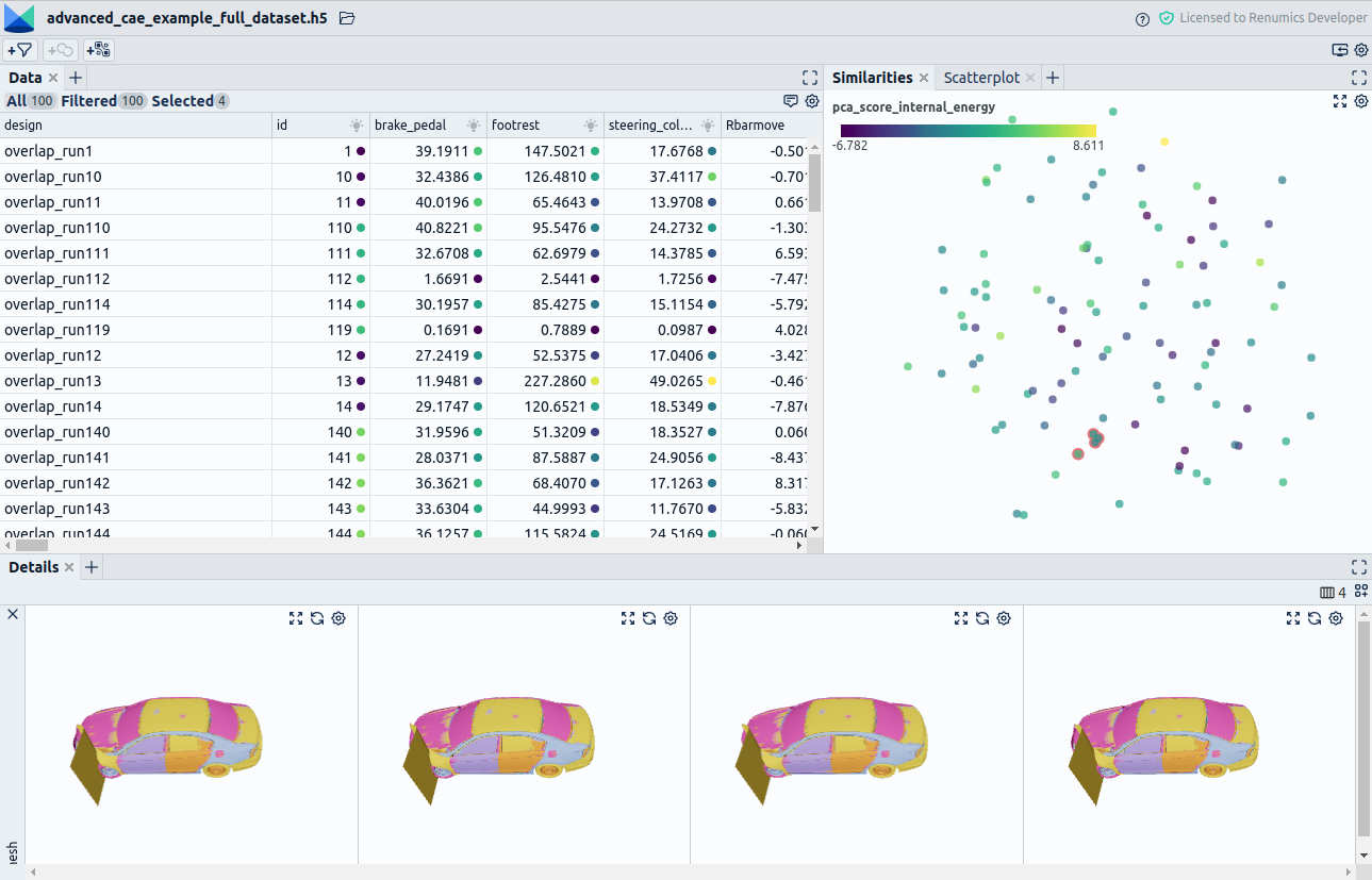
In this post, we thus show you how to optimize the selection of training samples in a data-driven way, demonstrating its viability on a realistic crash simulation dataset (Fig. 1).

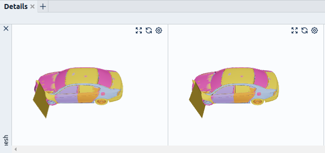
Our concrete goal is to build a surrogate model for the simulation of a car's crashworthiness (a car's ability to protect its occupants in a car crash). Our model would enable us to quickly explore the design space and select only the best designs for real-world testing. However, our dilemma is that building the model for replacing simulation runs requires running simulations for training purposes in the first place. Those can be very expensive! In our case, one simulation takes 9 hours to complete and needs about 20 GB for storing the results. So we really want to choose our simulation runs wisely.
Methodology
Our approach for building the surrogate model thus follows an iterative, "active learning-like" approach (Fig. 2).

This approach also follows ideas from data-centric AI, where instead of performing extensive hyperparameter optimization of your model, you try to iterate on your data instead.
Concretely we proceed as follows. We first train a probabilistic model on a limited set of simulation runs (56 runs). The model takes 27 input parameters as input variables, such as the sheet thickness of different car parts. The target value the model tries to predict is a value that determines if the relevant intrusion values are below a certain threshold.
We evaluate the model on a small validation set of 14 simulation runs with given intrusion annotations and visualize the results. Additionally, we evaluate the model on around 500 not yet executed simulations. From these 500 simulations, we want to choose the most valuable examples to improve our model in the following training iteration. We will then run simulations for those promising input parameters to generate intrusion value annotations to train the model.
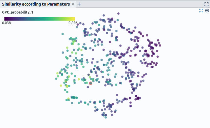
Concretely we set up the following visualization. We place the simulations with known intrusion values and the not yet executed (so unlabeled simulations) ones on a dimensionality reduction plot (Fig. 3).

The values we place by are the input parameters of the simulation that we consider relevant for deciding on the crashworthiness. Simulations with similar parameters should thus be closer together in the plot. Like this, we get some intuition on how the not yet run simulations relate to the ones where we know the intrusion values. We can now look at the evaluation result of these known simulations to make decisions on unknown simulations close by. Concretely we account for two things to make a decision which runs we should execute next:
- For which examples of the small test-set did the model make wrong predictions.
- For which not yet annotated examples did the model yield a high uncertainty value (see also Fig. 3).
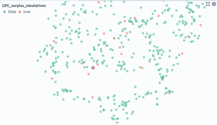
We can visualize these properties in our dimensionality reduction plots by introducing two additional dimensions via simple visualization techniques. Precisely, we can color or scale the data points according to different properties such as prediction correctness or model uncertainty. We mark not yet executed simulations close to misclassified or uncertain known simulation results to be run next (Fig. 4).

We then retrain on the selected runs and evaluate the gain in model performance. We compare this with a uniform, uninformed sample selection for testing purposes. As a result, we see the informed sample selection technique described above surpassing an uninformed sample selection. Concretely, our technique yields an over 5% higher gain in accuracy.
Conclusion
The previously described use case shows that going beyond quantitative metrics can lead to more robust surrogate models in simulation. Also, the procedure shown can lead to better data efficiency, saving hours of computations. Concretely, regarding typical problems in surrogate modeling, it significantly contributes to solving the sample selection problem. By selecting the simulations used for training the model in an iterative, informed way, you can substantially reduce the number of simulations needed for creating a robust model. The approach also shows that you can use new developments in machine learning to generate efficiency gains in simulation. The focus on data curation and data efficiency propagated by the data-centric AI movement helps reduce expensive label generation for surrogate modeling.
We hope that our article might inspire you also to consider trying out techniques like this in your simulation environment. If you are interested in the topic, feel free to get in touch or book a demo of our data curation tool Renumics Spotlight.
