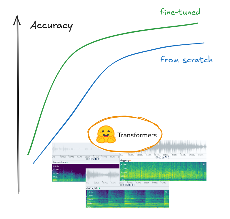
Fine-tuning an audio classification model instead of training from scratch can be more data efficient, leading to better results on the downstream task.
Introduction
Audio classification is one of the key tasks in audio understanding with Machine Learning and serves as a building block for many AI systems. It powers industry applications for test data evaluation in the engineering domain, error and anomaly detection, or predictive maintenance. Pre-trained transformer models, like the Audio Spectrogram Transformer (AST), provide a powerful foundation for these applications, offering robustness and flexibility.
While training an AST model from scratch would require a huge amount of data, using a pretrained model that has already learned audio-specific features can be more efficient. Fine-tuning these models with data specific to our use case is essential to enable their use for our particular application. This process adapts the model's capabilities to the unique characteristics of our dataset, such as classes and data distribution, ensuring the relevance of the results.
The AST model, integrated with the HuggingFace 🤗 Transformers library, has become a popular choice due to its ease of use and strong performance in audio classification tasks. This guide will take us through the entire process of fine-tuning a pretrained AST model (MIT/ast-finetuned-audioset-10–10–0.4593) using our own data, demonstrated with the ESC50 dataset. Using tools from the Hugging Face ecosystem and PyTorch as the backend, we will cover everything from data preparation and preprocessing to model configuration and training.
This tutorial will guide us through the process of fine-tuning the AST on our own audio classification dataset with tooling from the Hugging Face ecosystem. We will load the data (1), preprocess the audios (2), setup audio augmentations (3), configure and initialize the AST model (4) and finally, configure and start a training (5).
Step-by-Step Guide to Fine-Tune the AST
Before we start, install all the required packages with pip:
pip install transformers[torch] datasets[audio] audiomentations
1. Load Your Data in the Correct Format
To start, we'll use the Hugging Face 🤗 Datasets library to manage our data. This library will assist us in preprocessing, storing, and accessing data during training, as well as performing waveform transformations and encoding into spectrograms on the fly.
Our data should be loaded into a Dataset object with the following structure:
Dataset({
    features: ['audio', 'labels'],
    num_rows: 1234
})
In the following two sections I will demonstrate how to load a prepared dataset from the 🤗 Hub and also create a
Datasetfrom local audio data and labels.
Loading a Pre-existing Dataset from the HuggingFace Hub: If we don't have an audio dataset locally, we can conveniently load one from the Hugging Face Hub using the load_dataset function.
In this guide we will load the ESC50 Audio Classification dataset for demonstration purposes:
from datasets import load_dataset

esc50 = load_dataset("ashraq/esc50", split="train")
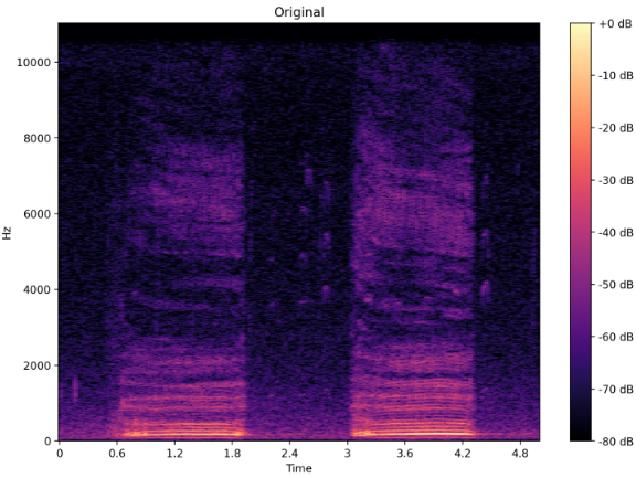
 Spectrograms of the audio samples from the ESC50 Dataset. Image from GitHub.
Loading Audio Files and Labels: We can load our audio files and associated labels into a Dataset object using a dictionary or a pandas DataFrame that contains file paths and labels. If we have a mapping of class names (strings) to label indices (integers), this information can be included during dataset construction.
Here's a practical example:
from datasets import Dataset, Audio, ClassLabel, Features

# Define class labels
class_labels = ClassLabel(names=["bang", "dog_bark"])

# Define features with audio and label columns
features = Features({
    "audio": Audio(),  # Define the audio feature
    "labels": class_labels  # Assign the class labels
})

# Construct the dataset from a dictionary
dataset = Dataset.from_dict({
    "audio": ["/audio/fold1/7061-6-0-0.wav", "/audio/fold1/7383-3-0-0.wav"],
    "labels": [0, 1],  # Corresponding labels for the audio files
}, features=features)
In this example:
- The
Audiofeature class automatically handles audio file loading and processing. ClassLabelhelps manage categorical labels, making it easier to handle classes during training and evaluation.
Note: For more information on loading audio with Hugging Face, have a look at the Datasets library Docs.
Inspecting the Dataset: Once the dataset is created, the audio data is recognized as an Audio feature, allowing for efficient access of the audio files. This means that data is loaded into memory only when needed, saving resources.
To inspect a data sample, use the following command:
print(dataset[0])
Output example:
{'audio': {'path': '/audio/fold1/7061-6-0-0.wav',
  'array': array([0.00000000e+00, 0.00000000e+00, 0.00000000e+00, ...,
         1.52587891e-05, 3.05175781e-05, 0.00000000e+00]),
  'sampling_rate': 44100},
 'labels': 0}
This output shows the path, waveform data array, and the sampling rate for the audio file, along with its corresponding label.
For the following steps, you can either use a prepared dataset as demo like we do or continue with your own dataset.
2. Preprocess the audio data
If our dataset is from the Hugging Face Hub, we cast the "audio" and "labels" columns to the correct feature types:
import numpy as np
from datasets import Audio, ClassLabel

# get target value - class name mappings
df = esc50.select_columns(["target", "category"]).to_pandas()
class_names = df.iloc[np.unique(df["target"], return_index=True)[1]]["category"].to_list()

# cast target and audio column
esc50 = esc50.cast_column("target", ClassLabel(names=class_names))
esc50 = esc50.cast_column("audio", Audio(sampling_rate=16000))

# rename the target feature
esc50 = esc50.rename_column("target", "labels")
num_labels = len(np.unique(esc50["labels"]))
In this code:
- Audio Casting: The
Audiofeature handles loading and processing audio files, resampling them to the desired sampling rate (16kHz in this case, sampling rate of theASTFeatureExtractor). - ClassLabel Casting: The
ClassLabelfeature maps integers to labels and vice versa.
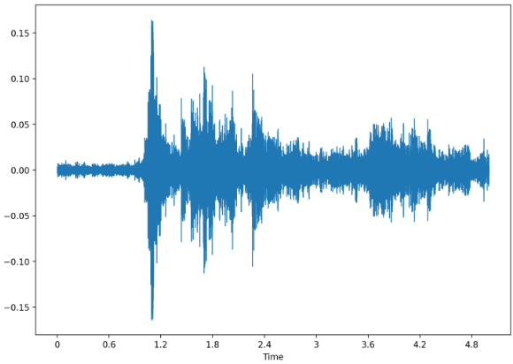
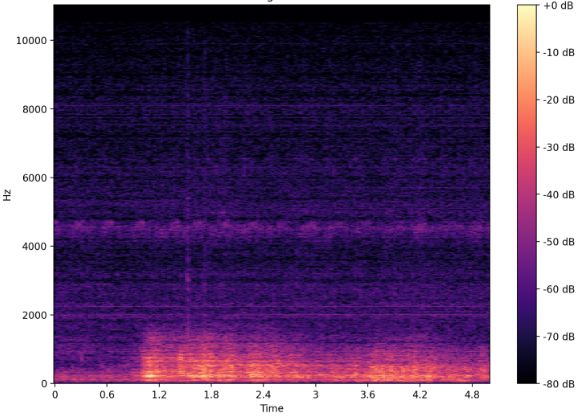 An audio array as waveform (upper) and as spectrogram (lower).
Preparing for AST Model Inputs: The AST model requires spectrogram inputs, so we need to encode our waveforms into a format that the model can process. This is achieved using the ASTFeatureExtractor, which is instantiated from the configuration of the pretrained model we intend to fine-tune on our dataset.
from transformers import ASTFeatureExtractor

# we define which pretrained model we want to use and instantiate a feature extractor
pretrained_model = "MIT/ast-finetuned-audioset-10-10-0.4593"
feature_extractor = ASTFeatureExtractor.from_pretrained(pretrained_model)

# we save model input name and sampling rate for later use
model_input_name = feature_extractor.model_input_names[0]  # key -> 'input_values'
SAMPLING_RATE = feature_extractor.sampling_rate
Note: It is important to set the mean and std values for normalization in the feature extractor to the values of our dataset. We can calculate the values using the following block of code:
# calculate values for normalization
feature_extractor.do_normalize = False  # we set normalization to False in order to calculate the mean + std of the dataset
mean = []
std = []

# we use the transformation w/o augmentation on the training dataset to calculate the mean + std
dataset["train"].set_transform(preprocess_audio, output_all_columns=False)
for i, (audio_input, labels) in enumerate(dataset["train"]):
    cur_mean = torch.mean(dataset["train"][i][audio_input])
    cur_std = torch.std(dataset["train"][i][audio_input])
    mean.append(cur_mean)
    std.append(cur_std)

feature_extractor.mean = np.mean(mean)
feature_extractor.std = np.mean(std)
feature_extractor.do_normalize = True
Applying Transforms for Preprocessing: We create a function to preprocess the audio data by encoding the audio arrays into the input_values format expected by the model. This function is set up to be applied dynamically, meaning it processes the data on-the-fly as each sample is loaded from the dataset.
def preprocess_audio(batch):
    wavs = [audio["array"] for audio in batch["input_values"]]
    # inputs are spectrograms as torch.tensors now
    inputs = feature_extractor(wavs, sampling_rate=SAMPLING_RATE, return_tensors="pt")

    output_batch = {model_input_name: inputs.get(model_input_name), "labels": list(batch["labels"])}
    return output_batch

# Apply the transformation to the dataset
dataset = dataset.rename_column("audio", "input_values")  # rename audio column
dataset.set_transform(preprocess_audio, output_all_columns=False)
If we load a sample now, it will be transformed on the fly and the encoded audios are yielded as input_values:
{'input_values': tensor([[-1.2776, -1.2776, -1.2776,  ..., -1.2776, -1.2776, -1.2776],
         [-1.2776, -1.2776, -1.2776,  ..., -1.2776, -1.2776, -1.2776],
         [-1.2776, -1.2776, -1.2776,  ..., -1.2776, -1.2776, -1.2776],
         ...,
         [ 0.4670,  0.4670,  0.4670,  ...,  0.4670,  0.4670,  0.4670],
         [ 0.4670,  0.4670,  0.4670,  ...,  0.4670,  0.4670,  0.4670],
         [ 0.4670,  0.4670,  0.4670,  ...,  0.4670,  0.4670,  0.4670]]),
 'label': 0}
Splitting the Dataset: As last data preprocessing step, we split the dataset into a train and test-set while utilizing the labels for stratification. This ensures to maintain class distribution across both sets.
# split training data
if "test" not in dataset:
    dataset = dataset.train_test_split(test_size=0.2, shuffle=True, seed=0, stratify_by_column="labels")
3. Add audio augmentations
To create a set of audio augmentations, we use the Compose class from the Audiomentations library, which allows us to chain multiple augmentations.
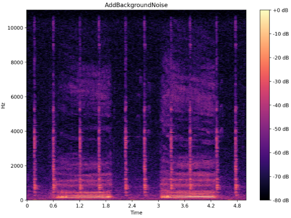 The original spectrogram of an audio file (upper) and the same audio with the AddBackgroundNoise transformation from Audiomentations library (lower).
Here's how to set it up:
from audiomentations import Compose, AddGaussianSNR, GainTransition, Gain, ClippingDistortion, TimeStretch, PitchShift

audio_augmentations = Compose([
    AddGaussianSNR(min_snr_db=10, max_snr_db=20),
    Gain(min_gain_db=-6, max_gain_db=6),
    GainTransition(min_gain_db=-6, max_gain_db=6, min_duration=0.01, max_duration=0.3, duration_unit="fraction"),
    ClippingDistortion(min_percentile_threshold=0, max_percentile_threshold=30, p=0.5),
    TimeStretch(min_rate=0.8, max_rate=1.2),
    PitchShift(min_semitones=-4, max_semitones=4),
], p=0.8, shuffle=True)
In this setup:
- The
p=0.8parameter specifies that each augmentation in theComposesequence has an 80% chance of being applied to any given audio sample. This probabilistic approach ensures variability in the training data, preventing the model from becoming overly dependent on any specific augmentation pattern and improving its ability to generalize. - The
shuffle=Trueparameter randomizes the order in which the augmentations are applied, adding another layer of variability.
For a better understanding of these augmentations and detailed configuration options, check out the Audiomentations' docs. Additionally, there's a great 🤗 Space where we can experiment with these audio transformations and hear and see their effects on the spectrograms.
Integrating Augmentations into the Training Pipeline: We apply these augmentations during the preprocess_audio transformation where we also encode the audio data into spectrograms.
The new preprocessing with augmentation is given by:
def preprocess_audio_with_transforms(batch):
    # we apply augmentations on each waveform
    wavs = [audio_augmentations(audio["array"], sample_rate=SAMPLING_RATE) for audio in batch["input_values"]]
    inputs = feature_extractor(wavs, sampling_rate=SAMPLING_RATE, return_tensors="pt")

    output_batch = {model_input_name: inputs.get(model_input_name), "labels": list(batch["labels"])}

    return output_batch

# Cast the audio column to the appropriate feature type and rename it
dataset = dataset.cast_column("audio", Audio(sampling_rate=feature_extractor.sampling_rate))
dataset = dataset.rename_column("audio", "input_values")
This function applies the defined augmentations to each waveform and then uses the ASTFeatureExtractor to encode the augmented waveforms into model inputs.
Setting Transforms for Training and Validation Splits: Finally, we set these transformations to be applied during the training and evaluation phases:
# with augmentations on the training set
dataset["train"].set_transform(preprocess_audio_with_transforms, output_all_columns=False)
# w/o augmentations on the test set
dataset["test"].set_transform(preprocess_audio, output_all_columns=False)
4. Configure and Initialize the AST for Fine-Tuning
To adapt the AST model to our specific audio classification task, we will need to adjust the model's configuration. This is because our dataset has a different number of classes than the pretrained model, and these classes correspond to different categories. It requires replacing the pretrained classifier head with a new one for our multi-class problem.
The weights for the new classifier head will be randomly initialized, while the rest of the model's weights will be loaded from the pretrained version. In this way, we benefit from the learned features of the pretraining and fine-tune on our data.
Here's how to set up and initialize the AST model with a new classification head:
from transformers import ASTConfig, ASTForAudioClassification

# Load configuration from the pretrained model
config = ASTConfig.from_pretrained(pretrained_model)

# Update configuration with the number of labels in our dataset
config.num_labels = num_labels
config.label2id = label2id
config.id2label = {v: k for k, v in label2id.items()}

# Initialize the model with the updated configuration
model = ASTForAudioClassification.from_pretrained(pretrained_model, config=config, ignore_mismatched_sizes=True)
model.init_weights()
Expected Output: We will see warnings indicating that some weights, especially those in the classifier layers, are being reinitialized:
Some weights of ASTForAudioClassification were not initialized from the model checkpoint at MIT/ast-finetuned-audioset-10-10-0.4593 and are newly initialized because the shapes did not match:
- classifier.dense.bias: found shape torch.Size([527]) in the checkpoint and torch.Size([2]) in the model instantiated
- classifier.dense.weight: found shape torch.Size([527, 768]) in the checkpoint and torch.Size([2, 768]) in the model instantiated
You should probably TRAIN this model on a down-stream task to be able to use it for predictions and inference.
5. Setup Metrics and Start Training
In the final step we will configure the training process with the 🤗 Transformers library and use the 🤗 Evaluate library to define the evaluation metrics to assess the model's performance.
Configure Training Arguments: The TrainingArguments class helps set up various parameters for the training process, such as learning rate, batch size, and number of epochs.
from transformers import TrainingArguments

# Configure training run with TrainingArguments class
training_args = TrainingArguments(
    output_dir="./runs/ast_classifier",
    logging_dir="./logs/ast_classifier",
    report_to="tensorboard",
    learning_rate=5e-5,  # Learning rate
    push_to_hub=False,
    num_train_epochs=10,  # Number of epochs
    per_device_train_batch_size=8,  # Batch size per device
    eval_strategy="epoch",  # Evaluation strategy
    save_strategy="epoch",
    eval_steps=1,
    save_steps=1,
    load_best_model_at_end=True,
    metric_for_best_model="accuracy",
    logging_strategy="steps",
    logging_steps=20,
)
Define Evaluation Metrics: Define metrics such as accuracy, precision, recall, and F1 score to evaluate the model's performance. The compute_metrics function will handle the calculations during training.
import evaluate
import numpy as np

accuracy = evaluate.load("accuracy")
recall = evaluate.load("recall")
precision = evaluate.load("precision")
f1 = evaluate.load("f1")

AVERAGE = "macro" if config.num_labels > 2 else "binary"

def compute_metrics(eval_pred):
    logits = eval_pred.predictions
    predictions = np.argmax(logits, axis=1)
    metrics = accuracy.compute(predictions=predictions, references=eval_pred.label_ids)
    metrics.update(precision.compute(predictions=predictions, references=eval_pred.label_ids, average=AVERAGE))
    metrics.update(recall.compute(predictions=predictions, references=eval_pred.label_ids, average=AVERAGE))
    metrics.update(f1.compute(predictions=predictions, references=eval_pred.label_ids, average=AVERAGE))
    return metrics
Setup the Trainer: Use the Trainer class from Hugging Face to handle the training process. This class integrates the model, training arguments, datasets, and metrics.
from transformers import Trainer

# Setup the trainer
trainer = Trainer(
    model=model,
    args=training_args,
    train_dataset=dataset["train"],
    eval_dataset=dataset["test"],
    compute_metrics=compute_metrics,  # Use the metrics function from above
)
Now that everything is set up, we can start training our model:
trainer.train()
6. (Not so optional:) Evaluate The Results
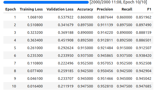
To understand our model's performance and find potential areas for improvement, it is essential to evaluate its predictions on train and test data. During training, metrics such as accuracy, precision, recall, and F1 score are logged to TensorBoard, which allows us to inspect the model's progress and performance over time. We can start tensorboard, by running tensorboard --logdir="./logs" in the shell.
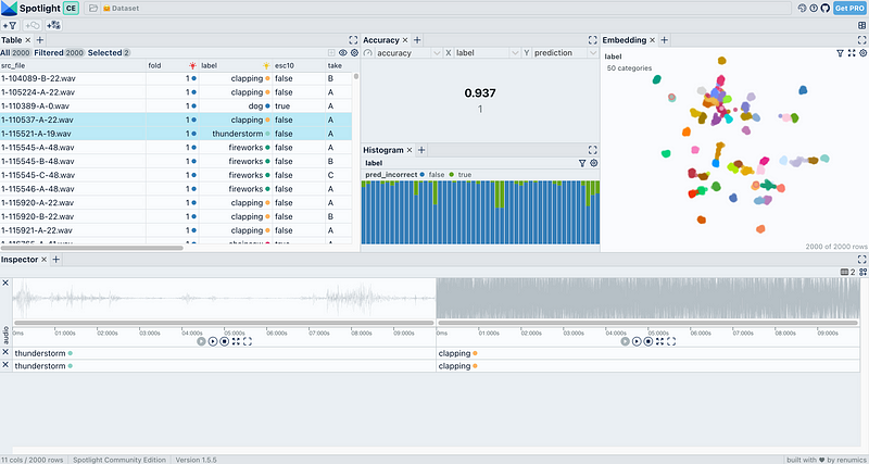 The ESC50 dataset with audio embeddings and model predictions loaded in Spotlight. Try it yourself in this Hugging Face Space.
For more detailed insights, we can inspect the model's predictions using Renumics' open-source tool, Spotlight. Spotlight enables us to explore and visualize the predictions alongside the data, helping us to identify patterns, potential biases, and miss-classifications on the level of single data points.
We can install Spotlight with pip:
pip install renumics-spotlight
And load the ESC50 dataset for interactive exploration with one line of code:
from renumics import spotlight

spotlight.show(esc50, dtype={"audio": spotlight.Audio})
This tutorial focuses on setting up the fine-tuning pipeline. For a comprehensive evaluation, including using Spotlight, please refer to the other tutorials and resources provided below and at the end of this guide (Useful Links).
Here are some examples of how to use Spotlight for model evaluation:
- A blog post with demo on Hands-On Voice Analytics with Transformers: Blog & 🤗 Space
- A blog post and short example on Fine-tuning image classification models from image search: Blog & Use Case
- A blog post and short example on How to Automatically Find and Remove Issues in Your Image, Audio, and Text Classification Datasets: Blog & Use Case
Conclusion
By following the steps outlined in this guide, we'll be able to fine-tune the Audio Spectrogram Transformer (AST) on any audio classification dataset. This includes setting up data preprocessing, applying effective audio augmentations, and configuring the model for the specific task. After training, we can evaluate the model's performance using the defined metrics, ensuring it meets our requirements. Once the model is fine-tuned and validated, it can be used for inference.
More on the Topic
This is the second in a series of tutorials and blog posts on the Audio Spectrogram Transformer for industrial audio classification use cases.
- Have a look at part one: How to Use SSAST Model Weigths in the HuggingFace Ecosystem? published in ITNEXT,
- and watch this list for upcoming posts.
Useful Links
- Download this guide as notebook from the Resource Page.
- A tutorial on how to use Spotlight for audio model evaluation: Link to Blog & 🤗 Space (Demo)
- A tutorial on how to train an acoustic event detection system with Spotlight: Link to Blog
- The official 🤗 audio course: Introduction & Fine-Tuning