Introduction
Acoustic event detection is crucial for automating tasks in various engineering use cases. Examples include the predictive maintenance of manufacturing machines and test data analysis in vehicle development. Depending on the use case, the goal of acoustic event detection is either to detect the presence of certain acoustic events in an audio recording or to determine the boundaries of the acoustic event's occurrence.
Recent progress in the area of acoustic event detection was primarily driven by advances in the area of Machine Learning and extensive research around topics such as conferencing systems and virtual assistants. However, challenges remain when tailoring these approaches to new, more specific use-cases. Here typically, the amount of available training data is comparatively small. Furthermore, the consistent annotation of the data through domain experts is costly and time-consuming.
This post shows how smart data labeling and Renumics Spotlight help overcome these challenges. We demonstrate how to train an acoustic event detection model with relatively few data points and speed up the annotation process while ensuring consistent labels over the whole dataset.
Building an acoustic event detection dataset
In our demonstration, we use a dataset consisting of around 8000 audio samples with a length of 1-4 seconds. Our goal is to train a model which accurately identifies audio samples containing siren noise. This goal could differ in a real-world use case from an engineering domain. An example would be identifying unpleasant noise occurring during a vehicle test drive.
To load the audio samples and associated metadata for annotation in Renumics Spotlight, we use the Renumics Backstage library. Backstage is a data preprocessing library written in Python specifically created to load a variety of complex data formats. These include common data types such as audio data, images, and more specific formats such as 3D meshes and simulation results.
import pandas as pd
from renumics.backstage import Dataset
from demo.utils import get_embedding, get_spectrogram

meta_data = pd.read_csv(“samples.csv”)

with Dataset(“dataset.h5”, “w”) as d:
 	d.from_pandas(meta_data)

    d.append_embedding_column("audio_embedding",  optional=True)
    d.append_audio_column("audio", optional=True)
    d.append_image_column("spectrogram", optional=True)

    for _, sample in df.iterrows():
        audio = get_audio(sample)
        d.append_row({
            “audio”: audio,
            “audio_embedding”: get_embedding(audio),
            “spectrogram”: get_spectrogram(audio)
        })
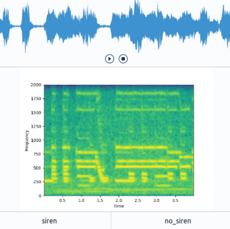
Here we create a dataset file and import tabular metadata of the audio samples from a CSV file. Additionally, we load audio data from disk and convert it into two more representations useful for annotating the dataset. Specifically, these are a spectrogram as easy to grasp visual representation and an audio embedding as a low dimensional representation suitable for similarity comparisons.
Labeling an initial set of samples using audio embeddings and metadata
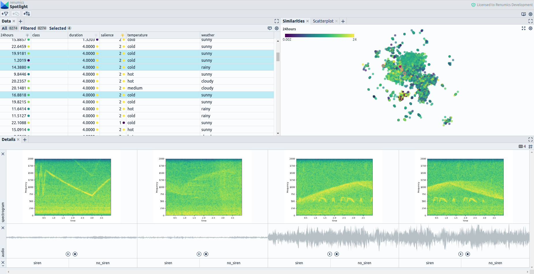
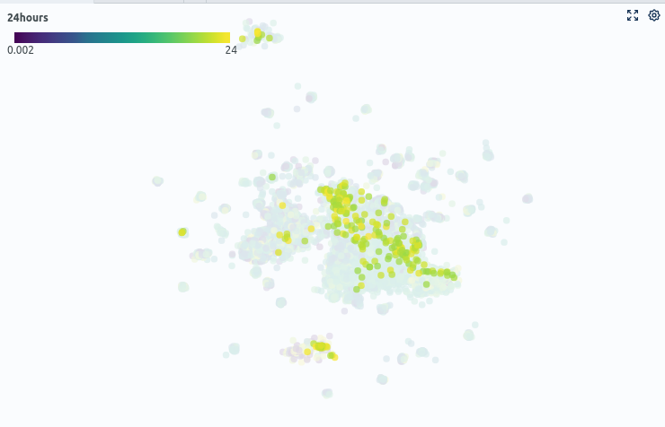
When opening the dataset in Spotlight, we see a table view of our data containing information over scalar metadata such as the duration of an audio snippet, the time of recording, or the corresponding weather conditions (Fig. 2). Also, we get a similarity map that uses the previously generated audio embeddings to show similarities between audio samples. Intuitively, data points close to each other are likely to be similar, while samples far from each other contain different kinds of audio events.
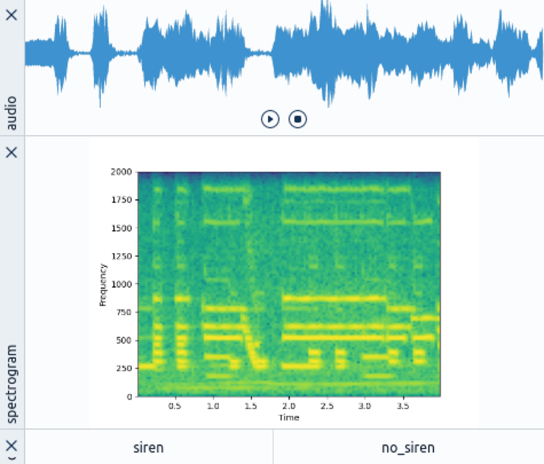
Additionally, we get a configurable view for a detailed qualitative assessment of each audio sample (Fig. 3). In this case, we configure Spotlight to show an audio player for playing back the audio sample, an image of the previously generated spectrogram, and a switch element for setting a label.
With the preconfigured labeling interface, we want to perform a first labeling round to train an initial model. Our first step is to identify which clusters in the similarity map are likely to contain siren noise. For that, we can easily use metadata. In this case, we filter out audio samples recorded after 8 pm under the hypothesis that siren noises are also present at night, unlike other sounds such as playing children. We also suspect siren noises to have a high saliency rating, so we use this as an additional filter criterion (Fig. 4). We then select samples from dense regions to identify a siren noise cluster.
In the initial labeling round, we label 15 siren samples and around 25 non-siren samples. By leveraging sample similarity shown on the similarity map, we are able to cover a wide variety of different siren sounds using a low number of labels. We then train a first classification model that uses the precomputed audio embedding for detecting sirens in the audio samples. From these simple steps, we already get a model that achieves a balanced accuracy score (average recall over classes) of 83%.
Leveraging model information for labeling
As a subsequent step, we show how to further optimize the model with informed decisions regarding the samples that should be labeled next. We do this by leveraging information about the initial model's classification performance. To do so, we first write information on the predictive performance of our model back to the dataset. We can now use additional information such as the entropy over the predicted probabilities to inform our decision on which samples to label next. The entropy here serves as a measure of uncertainty for model decisions.
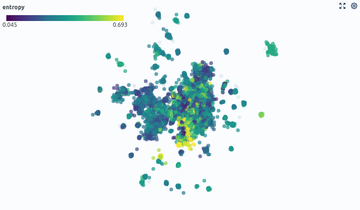
Using this information, we label 20 more samples (then having 60 annotated samples total) that fulfil two criteria:
- The model is uncertain (high entropy) when classifying the sample.
- According to the Similarity Map, the sample lies in an area with few labeled samples.
Evaluating the improved model
Following this simple annotation strategy, we get an increased balanced accuracy of about 88% and an F1-Score of around 0.81 in the siren class. These results correspond to an increase in balanced accuracy of 5 percentage points.
In contrast, on average, we reach a balanced accuracy of 80% when choosing the same number of samples uniformly. Also, here we have significantly more variance in model quality depending on which samples were uniformly chosen. An overview of how the informed labeling with Spotlight and the use of a pre-trained model affects the performance for this task is shown below.
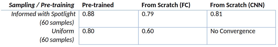
From the results (Fig. 6), one can see that informed labeling with Spotlight improves the performance of all types of models by at least 8% and by at least 19% when not using pre-trained models. In contrast, changing the model does lead to much smaller changes in performance. The results also show that informed labeling enables the training of certain model types with very few labels by improving the training stability. This stability is the result of the balancing of heterogeneous training examples. Regarding the use of pre-trained models, one can see that using pre-trained embedding models in conjunction with a smart selection of data samples achieves superior performance over all model configurations. Reaching the same balanced accuracy score of 0.88 would take 860 samples when training a fully connected neural network from scratch and >1000 samples for the convolutional neural network.
Summary
Summarizing the findings of our experiments informed labeling with Spotlight here benefits the model training in multiple ways:
- It enables a more balanced and less biased selection of training samples by letting us browse the dataset using different similarity metrics. This careful selection is essential when dealing with real-world datasets, which are often highly heterogeneous and unbalanced.
- It makes annotations more consistent by showing similar samples together, thus enabling detailed comparisons. Consistent annotations are a key factor to well-performing machine learning models.
- It allows us to incorporate information on model performance and uncertainty associated with specific data points. This additional information enables us to make informed decisions in our annotation process specific to the model's needs.
- It allows us to quickly inspect the dataset as well as model predictions visually to identify data- and model-related problems effectively.
- Spotlight works well together with most state-of-the-art embedding models such as transformers in NLP. It lets us compare pre-trained models to facilitate annotation and use them as a basis for model training.
Contact us to book a demo if you are interested in getting a live demonstration of this use case and talking about the benefits you might gain from using Spotlight.