The availability of benchmark datasets is one big reason for the impressive pace at which new machine learning methods are developed. This is a great situation that is envied by many disciplines (when I did my PhD in medical engineering the lack of benchmarks was a huge research bottleneck at the time). However, the heavy optimization towards specific datasets also has its disadvantages. One danger is that the performance of the developed methods is only meaningful for a specific context (I highly recommend the paper "Do ImageNet Classifiers Generalize to ImageNet" by Recht et al. in this context). Most importantly, benchmark datasets encourage ML researchers to think in a model-centric paradigm: They iterate different model architectures on a fixed dataset that they often know very little about.
Data-centric machine learning
In real applications the situation is typically very different: New datapoints or labels can be acquired and a deep domain expertise about the features, relationships and segments in the data is often available. Thus, it is also possible to iterate on the data and not just on the model. In fact, it is often a good idea to focus most efforts on the data and not on the model. This approach is known as data-centric machine learning.
For an introduction into data-centric AI and an interesting case study in the context of image-based defect detection I highly recommend this presentation by Andrew Ng. In the following, we present a step-by-step example that illustrates how a data-centric perspective can be used to optimize a machine learning model for 3D object classification based on CAD data. We will start from an established benchmark dataset and show how to reduce the overall error by 27% and a class-specific error by 71% within an afternoon.
Use cases for 3D shape classification in engineering and manufacturing
Many tasks in mechanical engineering revolve around the 3D representation of a physical product. Naturally, understanding 3D shapes plays an important role in AI-assisted engineering. Relevant use cases that either use a shape classification or that are closely related to this task include:
- Manufacturability analysis: An ML algorithm estimates the manufacturability of a mechanical part based on its shape and the corresponding geometric features. These techniques are used in additive manufacturing or sheet metal designs, for example.
- Cost estimation: Based on the shape, corresponding geometric features and additional information from PLM and ERP data, the cost of the mechanical part is estimated. This use case can be applied to different manufacturing processes and brings tremendous value if used in an iterative design-to-cost workflow.
- Automated simulation setup: Automated simulation workflows for products with different variants sometimes require information about the part types and properties that are not available in the PLM system. These properties can be estimated with ML based on the shape and PLM metadata to build fully automated workflows.
- Collision assessment for DMU: In the context of the digital mockup (DMU), geometric collisions of mechanical parts must be classified into relevant (i.e. mistakes by the engineering team) and non-relevant events (i.e. screw and nut). A ML algorithm trained on 3D shape and PLM metadata can automate this task to save a lot of time.
- Part search: Re-using existing parts instead of designing new ones saves a lot of time and money. Machine learning based shape retrieval helps to find similar parts or even parts that fit the intent of the design engineer.
Dataset and baseline
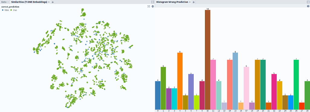
We start with the DMU-NET dataset that consists of 1916 CAD parts in 30 categories. We use a random split and train a PointNet++-based classifier on 958 parts. More details about the setup can be found in our upcoming paper "Data-Efficient Machine Learning on Three-Dimensional Engineering Data. A histogram shows that 126 out of 958 parts in the dataset are classified incorrectly (86.8% accuracy). This accuracy is in line with our published results and slightly better than the results reported by the original DMU paper that uses image-based methods.
Using a similarity map to gain insights into the model
A simple histogram reveals that the class cuttingtools (label class 10) is the worst-performing class: 14 out of 25 samples in the test set are classified incorrectly (Fig. 1 right). In the following, we will thus concentrate on the class for this showcase.
We use the TSNE method to map the embedding of the model to a 2D-space and create a scatter plot from the data (Fig. 1 left). In this visualization data points that the ML model regards as close together (in some metric that is induced by the loss) are grouped together on the 2D canvas. Hence, we call the plot a similarity map.
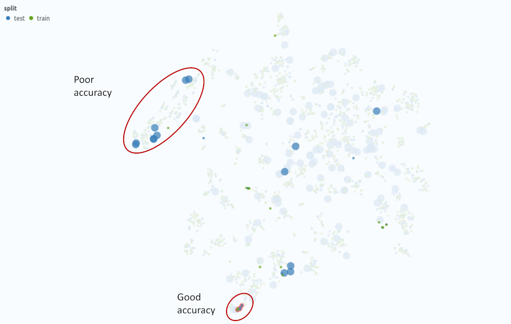
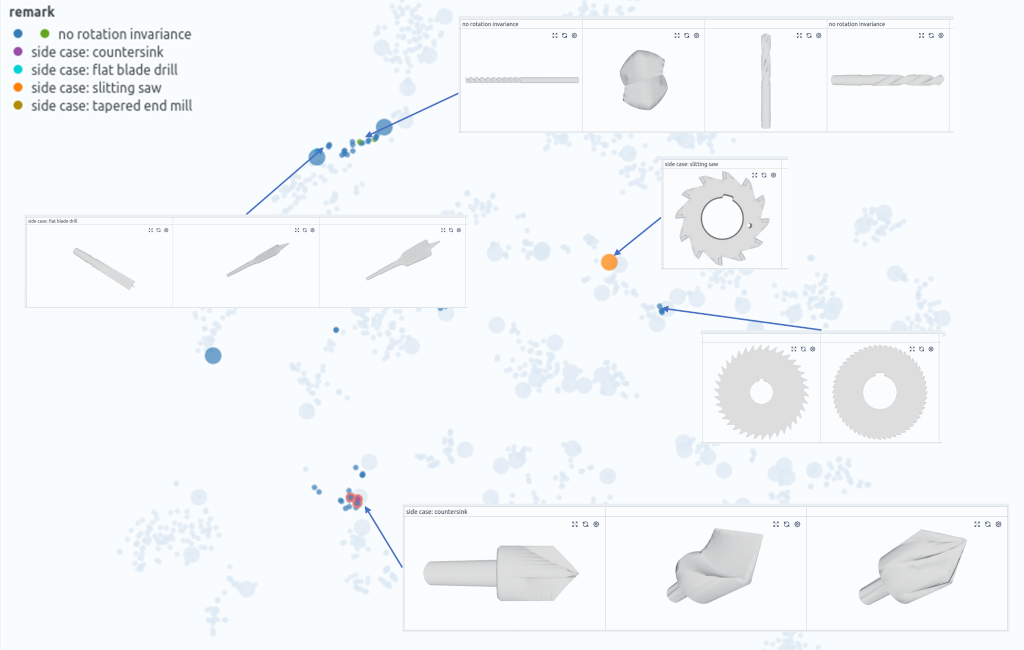
To further investigate the cuttingtool class, we filter out the corresponding data points. Then, we color the similarity map with the data split: Green points denote the training data, test data is colored blue (Fig. 2 right). We also scale the points with the result (small points denote correct predictions, large points incorrect predictions).
From this representation, we immediately note several things: First, the samples are distributed over the map. This indicates that the model is not able to identify common traits. Second, there exist a larger cluster with training and test samples, where the classification works well (Fig. 2), but there also is a cluster in the test set that is quite far away from the next training examples.
Determining the right normalization
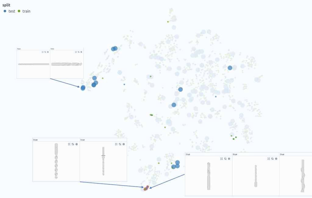
We now look at the individual datapoints in these clusters and quickly realize that the geometries itself are quite similar, but that the wrongly classified test samples are rotated by 90° (Fig. 3). We tag these samples and conclude that we should either augment our data with axis-aligned rotations or we should use a model that is invariant to this transformation.
Augmenting 3D data with different rotations or normalizing for rotation-invariance is a typical step in 3D shape classification. One could argue that you would iterate through different augmentation or normalization techniques in a model-centric workflow anyway. However, not only will this take a lot of computational time, but you might actually miss the best option. More concretely, augmenting the DMU dataset with random rotations or normalizing the main axis (e.g. with a principal component analysis) ahead of the training does not significantly change the overall performance. In contrast, we will see that specifically accounting for the axis-aligned rotations will indeed increase the accuracy.
In a real-world application, the similarity map along with a detailed view of several concrete examples goes a long way for optimizing the normalization of the model. This also helps in a debug scenario where the results are much worse than expected.
Identifying relevant side cases and populations
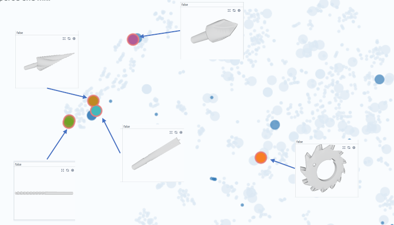
The similarity map reveals that there many different types of cutting tools in the dataset. Naturally, it is difficult for the model to generalize over these parts given the comparatively small overall training set size. We thus want to collect more datapoints for these unique tools. In an academic paper this would obviously be a cardinal sin, but in a real application it just simply is a good idea. So we channel our inner drilling and milling geek to identify and tag four tools that are not in the training set (Fig. 4):
- Tool #36: Countersink
- Tool #004: Flat-blade drill
- Tool #011: Tapered end mill
- Tool #13: Slitting saw
Even in this simple benchmark dataset, the step requires some domain expertise! When identifying side cases or outliers in a real engineering case, it is usually essential to discuss the samples or populations with the domain experts.

Enhancing the dataset and re-training
We use our insights to enhance the dataset in two ways: First, we download 3 additional parts from a vendor site for of the tools identified above. As we only check if the appearance is roughly similar to the edge cases, this just takes a couple of minutes. Next, we augment the dataset with additional axis-aligned rotations. Finally, we re-train our model. The histogram of the newly trained model reveals that we reduced the number of misclassified examples to 92. This means we have reduced the error by 27% and increased the accuracy to 90.4%. We also see that we only have 4 errors in the cutting tool class instead of 14 (71% reduction).
Now, let’s have a look at the similarity map again (Fig. 5). We notice that similar cutting tools that differ mainly by rotation are now grouped in the same cluster. We also observe the lonely test samples we identified are now grouped together with the respective tool type that we added to the training set. 3 out of 4 side cases are now identified correctly. Only the slitting saw case is still wrongly classified. It is apparent that the added models are not similar enough to the original geometry. This could easily be fixed in a subsequent iteration.
Model reliability and user trust
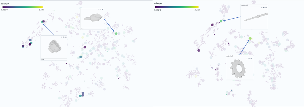
In most engineering applications, it is important to build tools that users can trust. In this context it is not necessarily a problem if a machine learning model fails as long as the model reports a low confidence along with the result. A simple metric for the confidence of the model is the entropy of the softmax prediction score. If we color our similarity map with this score, we realize that in the base model, only 2 out of 14 error cases have an entropy score larger than 2 (Fig. 6). In contrast, the re-retrained model assigns 2 out of 4 error cases a high entropy score. This in particular applies to the slitting saw side case. This means that while this side case is wrongly classified, we at least detect that this is a prediction with a high uncertainty. In a real application we can use this information to correct the prediction manually.
Conclusions
We showed how a data-centric approach allows to quickly enhance the accuracy of a ML model or 3D shape classification. To optimize the dataset, we used our data curation tool Renumics Spotlight. It helped us to include additional info from the model (embedding, confidence score) and allowed us to seamlessly switch between statistical information (e.g. histogram), aggregated views (e.g. similarity matrix) and individual examples. Thanks to this tooling, the described workflow can easily be completed in an afternoon.
Is data-centric ML a silver bullet? No, we still ended up with a model that makes mistakes. When running the model in production, it might still fail if the input distribution shifts too much. But: The data-centric approach allowed us to quickly improve the performance of the algorithm and to assess its reliability. In a real application, the benefits are typically even larger as the feature space and the different populations in the data are more complex.
Is data-centric ML completely new? No, every experienced data scientist knows that high-quality data is the most important building block for a good ML algorithm. Many data scientist actually spend a significant amount of time to build custom data curation, reporting and labeling tools. But: New data curation tools such as Renumics Spotlight allow data scientists and domain experts to quickly gain insight into larger datasets together. This helps to decrease model development time, to increase model performance, and to establish user trust.