Hands-On Voice Analytics with Transformers

tl:dr

Voice analytics has become an important part of AI systems and helps to build more sympathetic and more robust ML-based assistants. Pre-trained transformer models are a great starting point for voice AI. To make use of these models, systematic workflows for model debugging and comparison have to put in place. We implement basic strategies for a gender detection use case with the open source software packages Spotlight, sliceguard, audb and audonnx.

There is an interactive demo available.

Introduction

The human voice is an incredible expressive communication device. And it's not just what we say - it is how we say it. We can hear from the tone of the voice is somebody is sad or joyful, male or female and sometimes even if the person is healthy or not. Voice analytics seeks to determine these insights by using machine learning (ML) on voice recordings.

Voice analytics has become an important part of AI systems in many domains: Customer service, healthcare and academic research. Most importantly, voice analytics helps to build more sympathetic and more robust ML-based assistants.

Although the general field of voice analytics is quite broad, there are some core disciplines: Sentiment analysis as well as gender and age detection. In this blog, we show how to select a suitable pre-trained model for gender detection. In the process, we highlight useful strategies and open source tooling for modeling as well as model debugging and comparison.

Gender detection on the emodb dataset

In this tutorial, we use the emodb dataset. It is rich in metadata and easy to work with due to its small size. We install the necessary dependencies:

!pip install renumics-spotlight sliceguard audb audeer audformat audonnx audinterface

Then, we load the dataset with audb and take a first look at it by loading it into Spotlight:

import os
from renumics import spotlight
import audb
import audeer
import audformat


cache_root = audeer.mkdir('cache')

db = audb.load('emodb', version='1.3.0', format='wav', mixdown=True, sampling_rate=16000,
    full_path=False, cache_root=cache_root)

df = audformat.utils.concat([
    db['files'].get(map={'speaker': ['age', 'gender']}),
    db['emotion'].get(),
])
df['age'] = df['age'].astype('int')
df = df[['age', 'gender', 'emotion']]
df['audio'] = db.root + os.path.sep + df.index

#visualize it and hear some samples
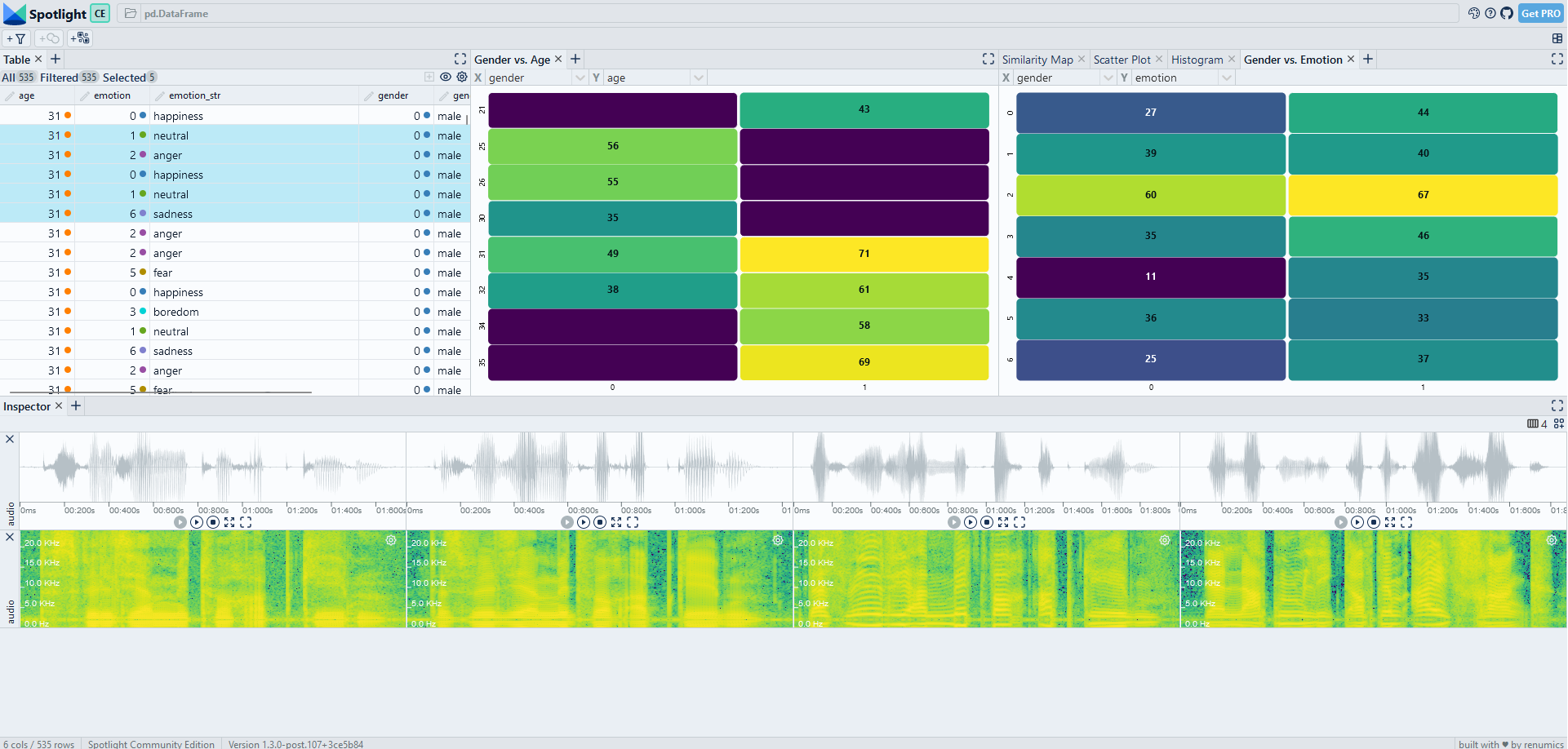
spotlight.show(df.reset_index())

Thanks to the interactive visualization, we can quickly familiarize ourselves with the dataset: It contains different phrases spoken by German stage actors. The actors deliver the phrase in different emotional states. For each delivery, the age and gender of the actor are given.

In a next step, we load a small pre-trained transformer model to predict each speaker's gender from the raw audio. We use the w2v2-L-robust-6-age-gender that is available through the audonnx package. The model is a stripped down version of a larger model that was trained on the aGender, Mozilla Common Voice, Timit and Voxceleb 2 datasets. We download the small transformer model:

model_name = 'gender_age_small'
model_url = 'https://zenodo.org/record/7761387/files/w2v2-L-robust-6-age-gender.25c844af-1.1.1.zip'

# def cache_model(model_root, cache_root, model_file, model_url):
def cache_model(model_name, model_url):

    model_root = audeer.path(cache_root, model_name)
    dst_path = audeer.path(cache_root, f'{model_name}.zip')

    if not os.path.exists(dst_path):
        audeer.download_url(model_url, dst_path, verbose=True)

    if not os.path.exists(model_root):
        audeer.extract_archive(dst_path, model_root, verbose=True)

# cache_model(model_root, cache_root, model_file, model_url)
cache_model(model_name, model_url)

And perform inference on the dataset:

import audonnx
import audinterface


def run_model(model_name, outputs):

    model_root = audeer.path(cache_root, model_name)
    model = audonnx.load(model_root)

    #handles pre-processing
    interface = audinterface.Feature(model.labels(outputs), process_func=model,
        process_func_args={'outputs': outputs, 'concat': True},
        sampling_rate=16000, resample=True, verbose=True)

    pred = interface.process_index(df.index, root=db.root,
        preserve_index=True, cache_root=model_root)

    return pred

outputs = ['logits_age', 'logits_gender', 'hidden_states']
pred = run_model(model_name, outputs)

Now we can take a look at the prediction results. As the audinterface class returns a dataframe with the logits, we have to compute the softmax probabilities and the predicted classes. We also use a pre-configured layout in Spotlight that gives us a good starting point for our model debugging process:

from scipy.special import softmax
from renumics.spotlight.layouts import debug_classification


df['m1_probabilities'] = pred[['female', 'male', 'child']].apply(softmax, axis=1)
df['m1_gender_prediction'] = pred[['female', 'male', 'child']].idxmax(axis=1).astype("category")
df['m1_embedding'] = pred.values.tolist()

layout = debug_classification(label='gender', prediction='m1_gender_prediction', embedding='m1_embedding', inspect={'audio': spotlight.Audio}, features=['age', 'emotion'])
spotlight.show(df.reset_index(), layout=layout)

Identifying voice AI failure modes

When we inspect the model results (interactive dataset available) we see that we reached an accuracy of 95.7%. That sounds not too bad. However, once we use the confusion matrix to drill into the data, we can identify two critical data slices (see Fig. 2): Most of the failures occurr in the slice [female, anger] while the slice [male, happiness] is also important. Concretely, on the [female, anger] slice the accuracy drops to 71.6%.

Having identified those slices, we typically have many options in a real-world use case to improve our AI system: We can collect more data similar to the slice, we can change features or normalization or we can just constrain our system to not operate in the problematic condition.

However, in a real-world datasets for voice AI, identifying such slices is much harder than on emodb. There are two reasons for this: There often is metadata available, but it is often unclear which metadata is meaningful at all. Also, expressive metadata (emotion in this case) is often lacking. Here, we demonstrate two strategies that can help in these situations:

Automatic slice detection algorithms can quickly identify candidates for data slices. We can use sliceguard to perform this on emodb:

from sliceguard import SliceGuard
from sklearn.metrics import accuracy_score
import numpy as np

sg = SliceGuard()

sg.find_issues(df, features=['emotion', 'age', 'gender'], y='gender', y_pred='m1_gender_prediction',
                        metric=accuracy_score, min_support=10, min_drop=0.15)

df_slices, issues, dtypes, sg_layout  = sg.report(no_browser=True)

spotlight.show(df.reset_index(), issues=issues, layout=layout)

Sliceguard identifies 8 slices. When we inspect these, we identify some spurious findings, but also the two critical slices [female, anger] and [male, happiness] that we already know.

In practice, the combination of data slice mining techniques with interactive inspection is a powerful way to uncover data patterns and model failure modes quickly.

The metadata information available in emodb with respect to age and emotion was very helpful for finding our data slices. What if this information is not available?

One option is to enrich the data by deploying other pre-trained models. In our case we use a pre-trained emotion detection model and compute an emotion embedding for each data sample:

model_name = 'emotion'
model_url = 'https://zenodo.org/record/6221127/files/w2v2-L-robust-12.6bc4a7fd-1.1.0.zip'

cache_model(model_name, model_url)

outputs = ['hidden_states']

pred_emo = run_model(model_name, outputs)
df['emotion_embedding'] = pred_emo.values.tolist()

Before we manually inspect the embedding, we compute slice candidates with sliceguard directly on the embedding:

sg = SliceGuard()


sg.find_issues(df, features=['embedding', 'gender'], y='gender', y_pred='m1_gender_prediction',
                        metric=accuracy_score, min_support=10, min_drop=0.15, precomputed_embeddings={'embedding': pred_emo.values})

df_slices, issues, dtypes, sg_layout  = sg.report(no_browser=True)

spotlight.show(df.reset_index(), issues=issues, layout=layout)

We see that the identified clusters on the embedding do primarily contain the [female, anger] slice, but that there are some other data samples from the happiness and fear emotions as well (Fig. 3). As expected, the embedding-based slice does not distinguish sharply between the metadata categories. However, it still helps to understand the underlying failure mode of the model.

Managing the trade-off between model size and performance

Some applications of voice analytics require the model to run on an edge device in real-time. In these use cases, model size matters a lot. There different strategies available to build smaller models: Quantization, pruning or knowledge distillation. Some of these techniques can be combined and each comes with its own trade-offs in terms of accuracy.

One key task in this scenario is to compare different models and find the right trade-off between size and accuracy. Here, global metrics alone are also not enough to judge the robustness of the model. Instead, the comparison has to be done a more fine-granular, slice-based level. Furthermore, the optimal trade-off heavily depends on the specific requirements of the use case. This means, these fine granular findings have to be reviewed with domain experts.

Here, we briefly show how to compare two differently-sized models for gender detection on emodb. We download and run a 12-layer transformer model for gender detection:

from renumics.spotlight.layouts import compare_classification

model_name = 'gender_age_big'
model_url = 'https://zenodo.org/record/7761387/files/w2v2-L-robust-24-age-gender.728d5a4c-1.1.1.zip'

cache_model(model_name, model_url)

outputs = ['logits_age', 'logits_gender', 'hidden_states']
pred = run_model(model_name, outputs)

df['m2_probabilities'] = pred[['female', 'male', 'child']].apply(softmax, axis=1)
df['m2_gender_prediction'] = pred[['female', 'male', 'child']].idxmax(axis=1)
df['m2_embedding'] = pred.values.tolist()

#compare models with Spotlight
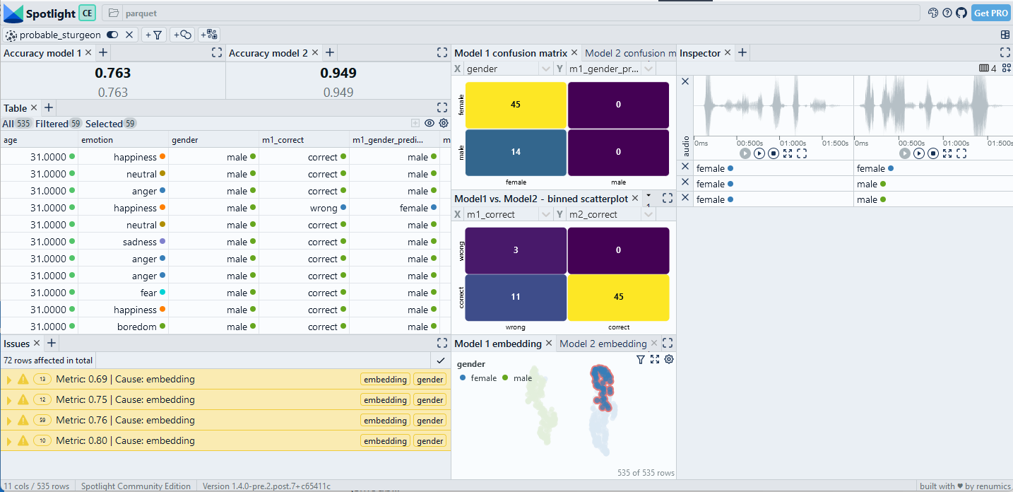
layout = compare_classification(label='gender', model1_prediction='m1_gender_prediction', model1_embedding='m1_embedding', model1_correct='m1_correct', model2_prediction='m2_gender_prediction', model2_embedding='m2_embedding', model2_correct='m2_correct', inspect={'audio': spotlight.Audio})
spotlight.show(df.reset_index(), issues=issues, layout=layout)

A very simple way to compare the model results is to look at the confusion matrix of model errors (Fig. 4). In this case, we see that the larger model strictly makes less mistakes than the smaller one. We also see that the errors in the slice [female, anger] are reduced from 19 to 4, raising the accuracy from 71.6% to 94%.

Conclusions

We have shown how to use and analyze pre-trained models for gender detection. These data-centric methods provide a good starting point for real-world applications on custom data and fine-tuned models. They also generalize to other voice analytics use cases such as sentiment analysis.

The code examples can be run on custom data and are based on the following open source tools:

• Spotlight for interactive visualization and curation.

• sliceguard to detect critical data slices.

• audb to work with audio datasets.

• audonnx for accessing pre-trained models.

Remarks

While voice AI is a very useful technology that has many benefits, it does not come without several important ethical implications. That is especially true for applications that deal with gender detection. I can recommend this review paper by Seymour et al. for a review on the topic.