tl:dr
Data slices are semantically meaningful subsets of the data, where the model performs anomalously. When dealing with an unstructured data problem (e.g. images, text), finding these slices is an important part of every data scientist’s job. In practice this task involves a lot of individual experience and manual work. In this post, we present some methods and tools to make finding data slices more systematic and efficient. We discuss current challenges and demonstrate some hands-on example workflows based on open-source tooling.
An interactive demo based on the CIFAR100 dataset can be found here: https://huggingface.co/spaces/renumics/cifar100-sliceguard-demo
Introduction
Debugging, testing and monitoring artificial intelligence (AI) systems is hard. Most efforts in the software 2.0 development process is spent on curating high-quality data sets.
An important strategy for developing robust machine learning (ML) algorithms is to identify so called data slices. Data slices are semantically meaningful subsets where the model performs anomalously. Identifying and tracking these data segments is at the heart of every data-centric AI development process. It is also a core aspect for deploying safe AI solutions in domains such as healthcare and automated driver assistance systems. Traditionally, finding data slices has been an integral part of a data scientist’s work. In practice, finding data slices heavily relies on the individual experience and domain knowledge of the data scientist. In the wake of the data-centric AI movement, there is a lot of current work and tooling that seek to make this process more systematic.
In this article, we give an overview over the current state of data slice finding on unstructured data. We specifically demonstrate some hands-on example workflows based on open-source tooling.
What is slice finding?
Data scientists use simple manual slice finding techniques all the time. The most famous example is probably the confusion matrix, a debugging method for classification problems. In practice, the slice finding process relies on a combination of pre-computed heuristics, the individual experience of the data scientist and a lot of interactive data exploration.
A classical data slice can be described by a conjunction of predicates on tabular features or metadata. In a people dataset this might be persons in a certain age range who are male and above 1.85m tall. In an engine condition monitoring dataset, a data slice might consist of data points in a certain RPM, operating hour, and torque range.
In the case of unstructured data, the semantic data slice definition can be more implicit: It can be a human understandable description such as “driving scenarios in light rain on a curvy road with heavy traffic in the mountains”.
Identifying data slices on unstructured dataset can be done in two different ways:
- Metadata can be extracted from the unstructured data either with classical signal processing algorithms (e.g. dark images, low SNR audio), or pre-trained deep neural networks for auto-tagging. Slice finding can then be done on this metadata.
- Latent representations in the embedding space can be used to group data clusters. These clusters can then be inspected to identify relevant data slices directly.
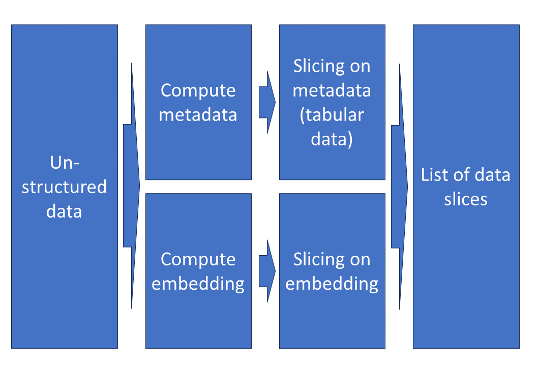 Fig. 1: Data slices on unstructured data can be computed on extracted metadata or based on model embeddings.
Automated slice finding techniques always seek to balance the support of the slice (should be large) with the severity of the model performance anomaly (should also be large).
Slice finding methods on tabular data share a lot of similarities with decision trees: In the context of ML model analysis, both techniques can be used to formulate rules that describe where model errors exist. However, there is one important difference: The slice finding problem allows for overlapping slices. This makes the problem computationally hard because it is more difficult to prune the search space.
Why is data slice finding important?
Especially within the last decade, the machine learning community did benefit tremendously from benchmark datasets: Starting with ImageNet, such datasets and competitions have been a big success factor for deep learning algorithms on unstructured data problems. In this context, the quality of a new algorithm is typically judged based on very few quantitative metrics such as F1-score or mean average precision.
With more and more ML models being deployed into production, it has become apparent that real-world datasets are very different from their benchmark peers: Real data is typically very noisy and imbalanced, but also rich in metadata information. For some use cases, cleaning and annotating these datasets can be prohibitively expensive.
Many teams have found that iterating the training dataset and monitoring drift in production is necessary to build and maintain safe AI systems. The idea of the data-centric AI movement is to provide methods and tools for systematically iterating datasets in a reliable, repeatable, and efficient way.
Finding data slices is a core part of this iteration process. Only by knowing where the model fails, it becomes possible to improve the system performance: By collecting more data, by correcting false labels, by selecting the best features or by simply restricting the operation domain of the system.
Why is data slice finding so difficult?
A critical aspect of slice finding is its computational complexity. We can illustrate this with a small example: Consider n binary features with one-hot encoding (can be obtained by binning or recoding, for example). Then the search space of all possible feature combination is O(2^n). This exponential nature means that heuristics are typically used for pruning. Consequently, automated slice finding not only takes quite long (depending on the number of features), but the output will not be an optimal stable solution, but some heuristics.
During the AI development process, poor model performance often stems from different root causes. Given the inherent stochastic nature of ML models, this can easily lead to spurious findings that have to be manually inspected and verified. Thus, even if a slice finding technique can produce a theoretically optimal result, it’s results must be manually inspected and verified. Building tools that allow cross-functional teams to this efficiently is a bottleneck for many ML teams.
We already stated that it is typically desirable to find slices with a large support, but also a distinct gap in model performance from the dataset baseline. Often, the relationships between different data slices are hierarchical in nature. Handling these hierarchies both during the automated slice finding process and during the interactive review phase is quite challenging.
Automated slice finding methods are most effective on metadata-rich problems. This is often the case for real-world problems. In contrast, Benchmark datasets are always quite sparse in metadata. Two primary reasons for this are data protection and anonymization requirements. With the lack of suitable example datasets, it is very difficult both to develop and to demonstrate effective slice finding workflows. We (unfortunately) must deal with this challenge in the following example section.
Hands-on: Finding data slices on CIFAR-100
The CIFAR-100 dataset is an established computer vision benchmark. We use it for this tutorial as its small size makes it easy to handle and keeps computational requirements low. The results are also easy to understand as they don’t require special domain knowledge.
Unfortunately, CIFAR-100 is already perfectly balanced, highly curated and lacks meaningful metadata. The results of the slice finding workflows we produce in this section are thus not as meaningful as in a real-world setting. In particular, we can’t benchmark the different tools against each other as the overall setting is too simplified. However, the presented workflows should be sufficient to understand how to quickly use them on your real-world data.
In a preparation step we compute image metadata with the Cleanvision library. More information on this enrichment can be found in our data-centric AI playbook.
Enriching images with metadata with Cleanvision
from cleanvision.imagelab import Imagelab
import pandas as pd
from renumics import spotlight
import requests

def cv_issues_cleanvision(df, image_name='image'):

    image_paths = df['image'].to_list()
    imagelab = Imagelab(filepaths=image_paths)
    imagelab.find_issues()

    df_cv=imagelab.issues.reset_index()

    return df_cv

dataset = datasets.load_dataset("renumics/cifar100-enriched", split="all")
df = dataset.to_pandas()

df_cv=cv_issues_cleanvision(df)
df = pd.concat([df, df_cv], axis=1)
We also define some important variables for our data slice analysis: The features to be analyzed as well as the names of the label and prediction columns:
from sklearn.metrics import accuracy_score

features=['dark_score', 'low_information_score', 'light_score', 'blurry_score', 'fine_label_str']
y_pred = 'fine_label_prediction'
y = 'fine_label'
error = 'fine_label_prediction_error'

accuracy_threshold = 0.75 * accuracy_score(df[y], df[y_pred])
Most slicing techniques only work on binned features. As the SliceLine and WisePizza libraries do not provide binning functionality themselves, we perform this as a pre-processing step:
from optbinning import ContinuousOptimalBinning
import numpy as np

optimal_binner = ContinuousOptimalBinning()
columns_to_bin = ["dark_score", "low_information_score", "light_score", "blurry_score"]

df_binned = df[features]
df_binned[columns_to_bin] = np.array([optimal_binner.fit_transform(df_binned[col], df[error], metric="bins") for col in columns_to_bin]).T
SliceLine
The Sliceline algorithm was proposed by Sagadeeva et al. in 2021. It is intended to work with large tabular datasets that contain many features. It leverages a novel pruning technique based on sparse linear algebra techniques and allows to find data slices quickly even on a single machine.
In this tutorial, we use the SliceLine implementation from the DataDome team. It runs very stable, but currently only supports Python versions <=3.9.
Most parameters of the SliceLine algorithm are very straight forward: The minimal support of the slice (min_sup), the maximum number of predicates to define a slice (max_l) and the maximum number of slices to be returned (k). The parameter alpha assigns a weight to the importance of the slice error and essential controls the trade-off between the size and the error drop-off of the slice.
We call the SliceLine library to get the 20 most interesting slices:
from slicefinder import Slicefinder


# fitting sliceline
sf = Slicefinder(
    alpha = 0.99,
    k = 20,
    max_l = 4,
    min_sup = 5,
    verbose = True
)

sf.fit(df_binned, df[error])
To interactively explore the slices, we enrich the description of each data slice:
Create data slice descriptions
from sklearn.metrics import accuracy_score
from renumics.spotlight.analysis.typing import DataIssue

#optional: sort slices by accuracy
accuracies = []

issues = []
for slice_index in range(len(sf.top_slices_)):
    current_slice = sf.top_slices_[slice_index]

    # create info for the slice
    feature_list=[feature_name for feature_name, feature_value in zip(sf.feature_names_in_, current_slice) if feature_value is not None]

    slice_info_string = ''.join([f"{feature_name}: {feature_value};" for feature_name, feature_value in zip(sf.feature_names_in_, current_slice) if feature_value is not None])

    # get slice element indices
    predicate_conditions = [df_binned[feature_name] == feature_value for feature_name, feature_value in zip(
        sf.feature_names_in_, current_slice) if feature_value is not None]
    condition = " & ".join([f"@predicate_conditions[{i}]" for i in range(len(predicate_conditions))])
    indices = df_binned.query(condition).index

    slice_accuracy = accuracy_score(df['fine_label'][indices], df['fine_label_prediction'][indices])
    if slice_accuracy < accuracy_threshold:
        severity = "high"
    else:
        severity = "medium"

    data_issue = DataIssue(
                severity=severity,
                title='Slice {0}: Accuracy: {1:2f}'.format(slice_index, slice_accuracy),
                description=slice_info_string,
                rows=indices.tolist(),
                columns=feature_list
            )

    issues.append(data_issue)
    accuracies.append(slice_accuracy)
We start Spotlight to explore the data slices interactively. You can directly experience the results in the Huggingface space.
Start interactive exploration with Spotlight
from renumics import spotlight
from renumics.spotlight import layout

#optional: sort issues
np_acc = np.array(accuracies)
sort_indices = np.argsort(np_acc)
issues = [issues[i] for i in sort_indices]

df_show = df.drop(columns=['embedding', 'probabilities'])
spotlight.show(
            df_show,
            dtype={"image": spotlight.Image, "embedding_reduced": spotlight.Embedding},
            issues=issues,
            layout=layout.layout(
                [
                    [layout.table()],
                    [layout.similaritymap()],
                    [layout.widgets.Issues()],
                ],
                [[layout.widgets.Inspector()]],
            ),
        )
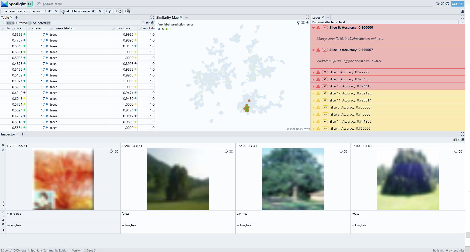
Fig. 2: Interactively exploring data slices generated by SliceLine. An interactive demo is available on Huggingface.
We see that the Sliceline algorithm did find some meaningful data slices in the CIFAR-100 dataset. The classes maple tree, willow tree and oak tree seem to be problematic. We also find that data points in these classes that have a high dark score are particularly challenging. Upon closer inspection we identify that this is because trees with a bright background are difficult for the model.
Wise Pizza
WisePizza is a recent development by the team from Wise. It is aimed at finding and visualizing interesting data slices in tabular data. The core idea is to use Lasso regression to find importance coefficients for each slice. More information on how Wise Pizza works can be found in the blog post.
It is important to note that WisePizza was not developed as a ML debugging tool. Instead, it is primarily aimed at supporting segment analysis during EDA. That is why it is possible to manually define segment candidates and assign a weight to them. In our experiments, we run WisePizza directly on the dataset and set the weight for each data point to 1:
from wise_pizza import explain_levels, explain_changes_in_totals, explain_changes_in_average

df_binned['count'] = 1
df_binned[error]=df[error]

sf = explain_levels(
    df=df_binned,
    dims=features,
    total_name=error,
    size_name='count',
    min_depth=1,
    max_depth=3,
    min_segments=20,
    solver="lasso"
)
sf.plot(width=500, height=100, plot_is_static=False)
WisePizza has built-in visualizations for tabular data. To explore our unstructured data set, we extract data slice descriptions to visualize in Spotlight:
Create data slice descriptions
from sklearn.metrics import accuracy_score
from renumics.spotlight.analysis.typing import DataIssue

#optional: sort slices by accuracy
accuracies = []

issues = []

for idx, slice in enumerate(sf.segments):
    slice_info_string = ''.join([f"{feature_name}: {feature_value}," for feature_name, feature_value in slice['segment'].items()])

    # get slice element indices
    predicate_conditions = [df_binned[feature_name] == feature_value for feature_name, feature_value in slice['segment'].items()]
    condition = " & ".join([f"@predicate_conditions[{i}]" for i in range(len(predicate_conditions))])
    indices = df_binned.query(condition).index

    slice_accuracy = accuracy_score(df['fine_label'][indices], df['fine_label_prediction'][indices])
    if slice_accuracy < accuracy_threshold:
        severity = "high"
    else:
        severity = "medium"


    data_issue = DataIssue(
                severity=severity,
                title='Slice {0}: Accuracy: {1:2f}'.format(idx, slice_accuracy),
                description=slice_info_string,
                rows=indices.tolist(),
            )

    issues.append(data_issue)
    accuracies.append(slice_accuracy)
Start interactive exploration with Spotlight
from renumics import spotlight
from renumics.spotlight import layout

#optional: sort issues
np_acc = np.array(accuracies)
sort_indices = np.argsort(np_acc)
issues = [issues[i] for i in sort_indices]

df_show = df.drop(columns=['embedding', 'probabilities'])
spotlight.show(
            df_show,
            dtype={"image": spotlight.Image, "embedding_reduced": spotlight.Embedding},
            issues=issues,
            layout=layout.layout(
                [
                    [layout.table()],
                    [layout.similaritymap()],
                    [layout.widgets.Issues()],
                ],
                [[layout.widgets.Inspector()]],
            ),
        )
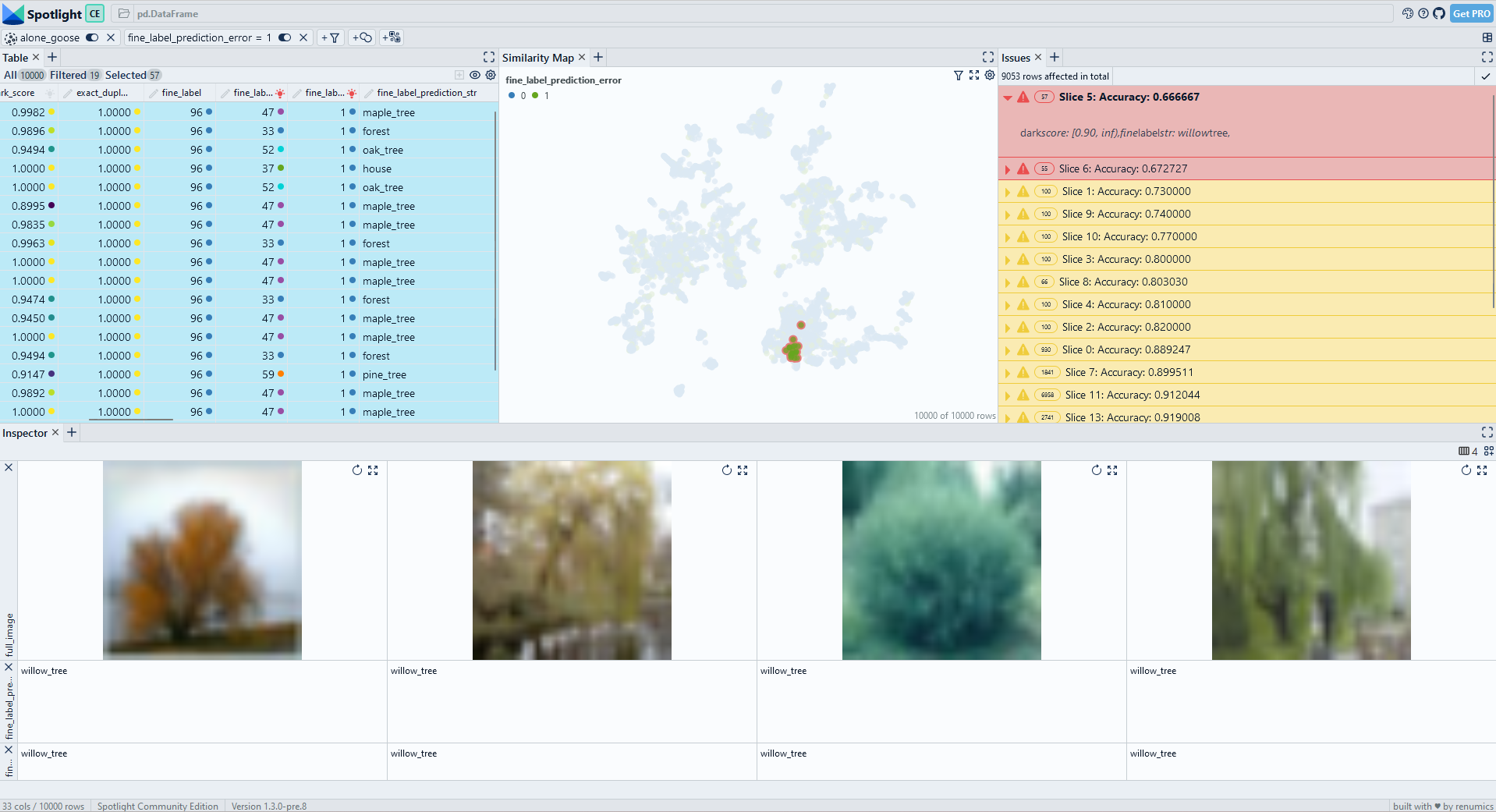 Fig. 3: WisePizza also identifies the willow tree class with large dark scores as problematic. However, the slices are not as fine-granular as the SliceLine results.
On the simple CIFAR-100 benchmark dataset, WisePizza finds relevant segments: It also lists the willow tree class with a high dark score as the top slice. However, the following results are limited to different class categories and are not as fine-granular as the SliceLine output. One reason is that the WisePizza algorithm does not directly provide a weighting mechanism between the support of the slice and the accuracy drop.
Sliceguard
The Sliceguard library uses hierarchical clustering to determine possible data slices. Then, methods from fair learning are used to rank these clusters and predicates are mined through explainable AI techniques. More information on Sliceguard can be found in this blog post by my colleague Daniel Klitzke.
The main reason we built Sliceguard is the fact that it not only works on tabular data, but also directly on embeddings. The library offers a lot of built-in functionality for pre-processing (e.g. binning) and post-processing.
We can run Sliceguard on CIFAR-100 with just a few lines of code:
from sklearn.metrics import accuracy_score

precomputed_embeddings = {'embedding': df['embedding'].to_numpy()}
    feature_types = {'dark_score': 'numeric', 'low_information_score': 'numeric',
    'light_score': 'numeric', 'blurry_score': 'numeric', 'fine_label': 'nominal' }

    sg = SliceGuard()
    issue_df = sg.find_issues(
        df,
        features,
        y,
        y_pred,
        accuracy_score,
        precomputed_embeddings = precomputed_embeddings,
        metric_mode="max",
        feature_types={'fine_label': 'nominal'}
    )
Sliceguard uses Spotlight to provide an interactive visualization of the identified data slices:
issue_df, issues = sg.report(spotlight_dtype={"image": Image})
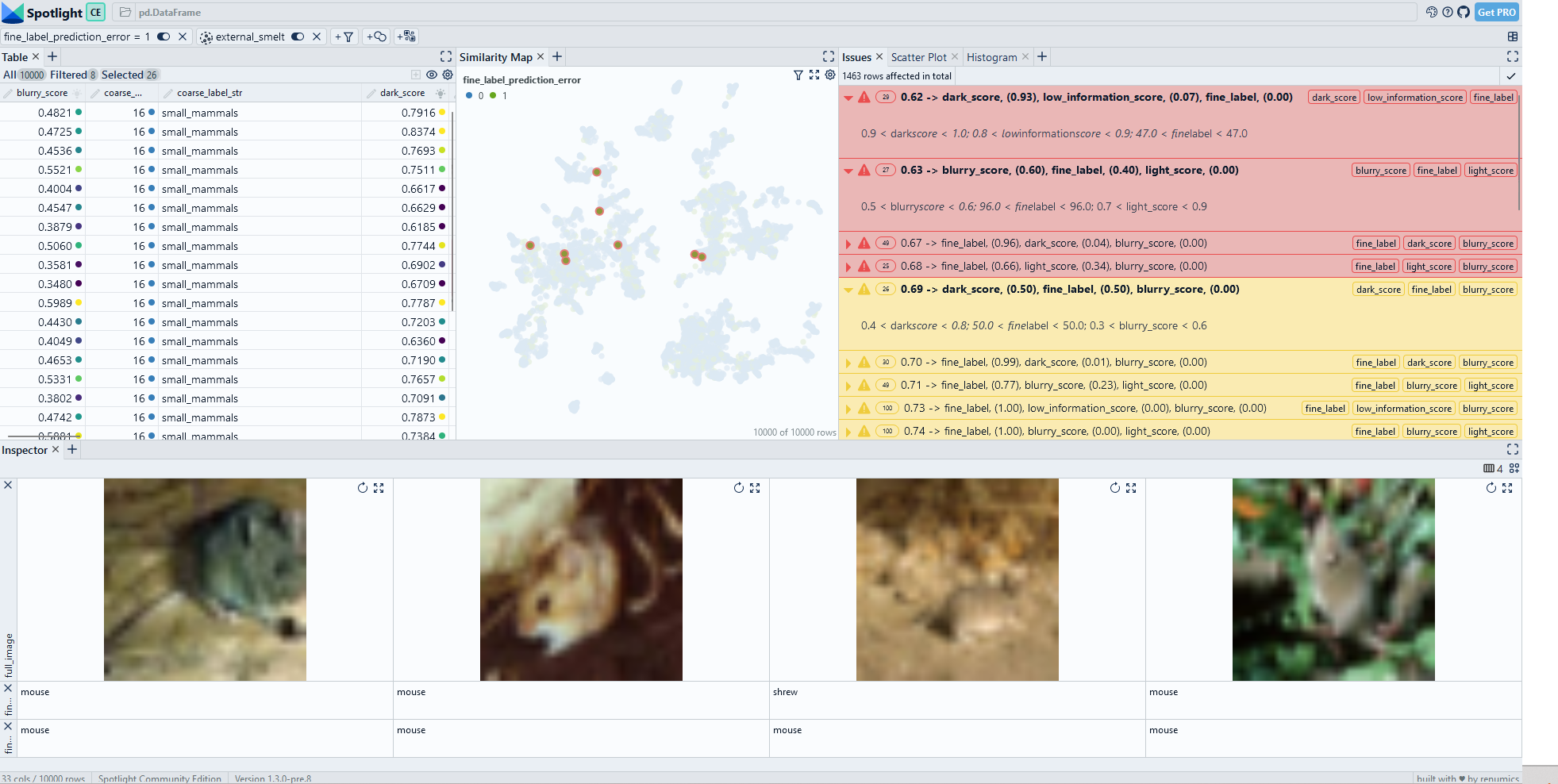
Sliceguard can uncover fine-granular data slices on the CIFAR-100 datset (Fig. 5). In addition to the previously discovered data slices in the tree categories, we also identify other issues (e.g. in the mouse class).
 Fig. 4: Sliceguard uncovers fine-granular data slices. An interactive demo is available on Huggingface.
Conclusions
We have presented three open source tools for mining data slices. Even on the simple CIFAR-100 benchmark, they can be used to uncover critical data segments quickly. Identifying these data slices is an important step to understand model failure modes and to improve the training dataset.
The SliceLine tool works on tabular data and identifies data slices that are described by a combination of predicates. Sliceguard does return a mathematically guaranteed optimal combination of predicates, but it can directly work with embeddings. Additionally, it can be run on unstructured data sets with just a few lines of code.
In practice, both SliceLine and Sliceguard are very helpful for identifying data slices. However, both tools cannot be used for a fully automated slice analysis. Instead, they provide powerful heuristics that can be combined with interactive exploration. If done correctly, this approach is an important tool for interdisciplinary data teams to build reliable ML systems.