
TL;DR
Fine-tuning significantly influences embeddings in image classification. Pre-fine-tuning embeddings offer general-purpose representations, whereas post-fine-tuning embeddings capture task-specific features. This distinction can lead to varying outcomes in outlier detection and other tasks. Both pre-fine-tuning and post-fine-tuning embeddings have their unique strengths and should be used in combination to achieve a comprehensive analysis in image classification and analysis tasks.
Checkout out one of the online Demos of the CIFAR-10 dataset [3] for this article:
Projection of embeddings with PCA during fine-tuning of a Vision Transformer (ViT) model [1] on CIFAR10 [3]; Source: created by the author.
1 Introduction
The use of pre-trained models on large datasets, such as ImageNet, followed by fine-tuning on specific target datasets, has become the default approach in image classification. However, when dealing with real-world target datasets, it is important to consider their inherent noise, which includes outliers, label errors, and other anomalies. Interactive exploration of datasets plays a crucial role in gaining a comprehensive understanding of the data, enabling the identification and resolution of critical data segments through the utilization of data enrichments.
Embeddings play a crucial role in analyzing unstructured image data. They provide high-level semantic information and support various tasks such as data analysis, insight generation and outlier detection. By representing images in a lower-dimensional space, embeddings make it easier to explore similarities and differences within the data and allows for the creation of similarity maps using techniques like t-SNE or UMAP. We will use Spotlight to interactively explore the enriched datasets we create:
Disclaimer: The author of this article is also one of the developers of Spotlight. Some of the code snippets in this article are also available in the Spotlight repository.
In this article, we will delve into the differences between pre and post fine-tuning embeddings, with an additonal focus on outlier detection. While it is important to note that using embeddings from fine-tuned models may not always yield the best results for outlier detection as we could also use the probabilities, it still presents an intriguing approach. The visualization of embeddings adds a visually appealing dimension to the analysis process.
To assess the performance and effectiveness of embeddings in outlier detection tasks, we will examine exemplary datasets that are widely used in image classification. Moreover, we will utilize two common foundation model. Through this exploration, we aim to gain insights into the effect of Model Fine-tuning on the embeddings, providing a better understanding of their capabilities and limitations.
2 Preparations
Install the required Python Packages:
!pip install renumics-spotlight datasets torch pandas cleanlab annoy
2.1 Extract Embeddings
We will use the following models based on google/vit-base-patch16–224-in21k [1] and microsoft/swin-base-patch4-window7–224 [2] available on Hugging Faces to extract pre-fine-tuning embeddings and the best-liked fine-tuned models for each dataset: araki/vit-base-patch16–224-in21k-finetuned-cifar10, MazenAmria/swin-tiny-finetuned-cifar100, nateraw/vit-base-beans, farleyknight/mnist-digit-classification-2022–09–04.
case = {
    "cifar10": {
        "base_model_name": "google/vit-base-patch16-224-in21k",
        "ft_model_name": "aaraki/vit-base-patch16-224-in21k-finetuned-cifar10",
    },
    "beans": {
        "base_model_name": "google/vit-base-patch16-224-in21k",
        "ft_model_name": "nateraw/vit-base-beans",
    },
    "mnist": {
        "base_model_name": "google/vit-base-patch16-224-in21k",
        "ft_model_name": "farleyknight/mnist-digit-classification-2022-09-04",
    },
    "cifar100": {
        "base_model_name": "microsoft/swin-base-patch4-window7-224",
        "ft_model_name": "MazenAmria/swin-tiny-finetuned-cifar100",
    },
}
To load the dataset, we utilize the load_dataset function from the datasets module and prepare it for the image classification task. You can choose from the tested and reported dataset of this article CIFAR-10 [3], CIFAR-100 [3], MNIST [4] and Beans [5] or try different image classification datasets from Hugging Face with corresponding models.
import datasets
# choose from cifar10, cifar100, mnist or beans.
# corresponding model will be selected automatically
DATASET = "cifar10"
ds = datasets.load_dataset(DATASET, split="train").prepare_for_task(
    "image-classification"
)
df = ds.to_pandas()
# df = df.iloc[:1000] # uncomment to limit the dataset size for testing
We define the huggingface_embedding function to extract embeddings from both the fine-tuned model and the base/foundation model. The embeddings are stored in separate columns ("embedding_ft" and "embedding_foundation") in the original dataframe (df):
import datasets
from transformers import AutoFeatureExtractor, AutoModel
import torch
import pandas as pd

ft_model_name = case[DATASET]["ft_model_name"]
base_model_name = case[DATASET]["base_model_name"]
def extract_embeddings(model, feature_extractor, image_name="image"):
    """
    Utility to compute embeddings.
    Args:
        model: huggingface model
        feature_extractor: huggingface feature extractor
        image_name: name of the image column in the dataset
    Returns:
        function to compute embeddings
    """
    device = model.device
    def pp(batch):
        images = batch[image_name]
        inputs = feature_extractor(
            images=[x.convert("RGB") for x in images], return_tensors="pt"
        ).to(device)
        embeddings = model(**inputs).last_hidden_state[:, 0].cpu()
        return {"embedding": embeddings}
    return pp

def huggingface_embedding(
    df,
    image_name="image",
    modelname="google/vit-base-patch16-224",
    batched=True,
    batch_size=24,
):
    """
    Compute embeddings using huggingface models.
    Args:
        df: dataframe with images
        image_name: name of the image column in the dataset
        modelname: huggingface model name
        batched: whether to compute embeddings in batches
        batch_size: batch size
    Returns:
        new dataframe with embeddings
    """
    # initialize huggingface model
    feature_extractor = AutoFeatureExtractor.from_pretrained(modelname)
    model = AutoModel.from_pretrained(modelname, output_hidden_states=True)
    # create huggingface dataset from df
    dataset = datasets.Dataset.from_pandas(df).cast_column(image_name, datasets.Image())
    # compute embedding
    device = "cuda" if torch.cuda.is_available() else "cpu"
    extract_fn = extract_embeddings(model.to(device), feature_extractor, image_name)
    updated_dataset = dataset.map(extract_fn, batched=batched, batch_size=batch_size)
    df_temp = updated_dataset.to_pandas()
    df_emb = pd.DataFrame()
    df_emb["embedding"] = df_temp["embedding"]
    return df_emb

embeddings_df = huggingface_embedding(
    df,
    modelname=ft_model_name,
    batched=True,
    batch_size=24,
)
embeddings_df_found = huggingface_embedding(
    df, modelname=base_model_name, batched=True, batch_size=24
)
df["embedding_ft"] = embeddings_df["embedding"]
df["embedding_foundation"] = embeddings_df_found["embedding"]
2.2 Calculate outlier score
Next we use Cleanlab to calculate outlier scores both the fine-tuned model and the base/foundation based on the embeddings. We utilize the OutOfDistribution class to compute the outlier scores. The resulting outlier scores are stored in the original dataframe (df):
from cleanlab.outlier import OutOfDistribution
import numpy as np
import pandas as pd
def outlier_score_by_embeddings_cleanlab(df, embedding_name="embedding"):
    """
    Calculate outlier score by embeddings using cleanlab
        Args:
            df: dataframe with embeddings
            embedding_name: name of the column with embeddings
        Returns:
            new df_out: dataframe with outlier score
    """
    embs = np.stack(df[embedding_name].to_numpy())
    ood = OutOfDistribution()
    ood_train_feature_scores = ood.fit_score(features=np.stack(embs))
    df_out = pd.DataFrame()
    df_out["outlier_score_embedding"] = ood_train_feature_scores
    return df_out

df["outlier_score_ft"] = outlier_score_by_embeddings_cleanlab(
    df, embedding_name="embedding_ft"
)["outlier_score_embedding"]
df["outlier_score_found"] = outlier_score_by_embeddings_cleanlab(
    df, embedding_name="embedding_foundation"
)["outlier_score_embedding"]
2.3 Find nearest neighbor
To evaluate the outliers, we calculate the nearest neighbor image with the Annoy library using the fine-tuned model only. The resulting images are stored in the original DataFrame (df):
from annoy import AnnoyIndex
import pandas as pd
def nearest_neighbor_annoy(
    df, embedding_name="embedding", threshold=0.3, tree_size=100
):
    """
    Find nearest neighbor using annoy.
    Args:
        df: dataframe with embeddings
        embedding_name: name of the embedding column
        threshold: threshold for outlier detection
        tree_size: tree size for annoy
    Returns:
        new dataframe with nearest neighbor information
    """
    embs = df[embedding_name]
    t = AnnoyIndex(len(embs[0]), "angular")
    for idx, x in enumerate(embs):
        t.add_item(idx, x)
    t.build(tree_size)
    images = df["image"]
    df_nn = pd.DataFrame()
    nn_id = [t.get_nns_by_item(i, 2)[1] for i in range(len(embs))]
    df_nn["nn_id"] = nn_id
    df_nn["nn_image"] = [images[i] for i in nn_id]
    df_nn["nn_distance"] = [t.get_distance(i, nn_id[i]) for i in range(len(embs))]
    df_nn["nn_flag"] = df_nn.nn_distance < threshold
    return df_nn

df_nn = nearest_neighbor_annoy(
    df, embedding_name="embedding_ft", threshold=0.3, tree_size=100
)
df["nn_image"] = df_nn["nn_image"]
2.4 Visualize
For visualization with Spotlight purposes, a new “label_str” column is created in the DataFrame by mapping integer labels to their string representations using a lambda function. The dtypes dictionary is used to specify the data type of each column to get the proper visualization, while the layout determines the arrangement and displayed columns in the visualization:
from renumics import spotlight
df["label_str"] = df["labels"].apply(lambda x: ds.features["labels"].int2str(x))
dtypes = {
    "nn_image": spotlight.Image,
    "image": spotlight.Image,
    "embedding_ft": spotlight.Embedding,
    "embedding_foundation": spotlight.Embedding,
}
spotlight.show(
    df,
    dtype=dtypes,
    layout="https://spotlight.renumics.com/resources//layout_pre_post_ft.json",
)
This will open a new browser window:
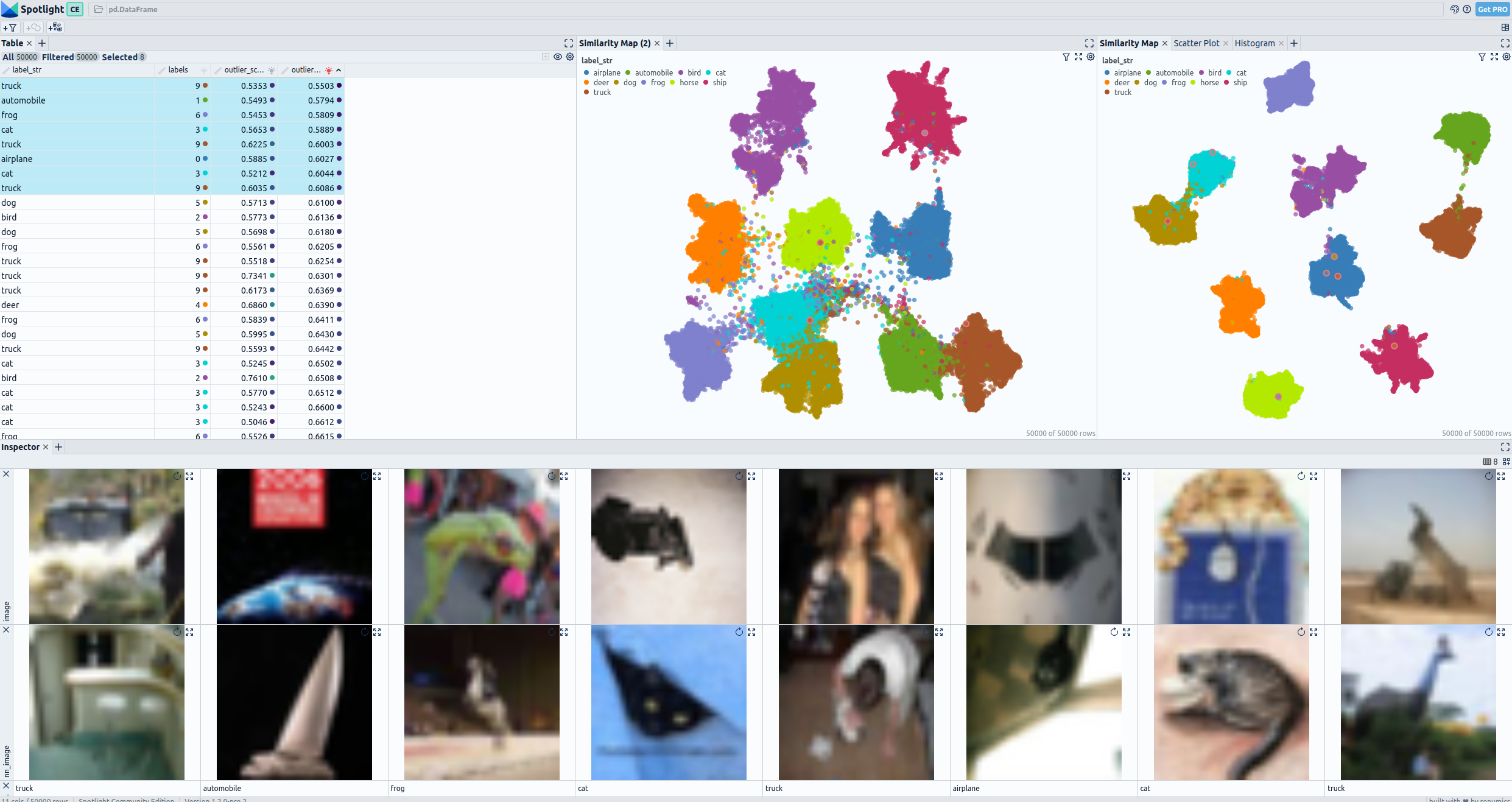
Pre and post fine-tuning embeddings for CIFAR-10: UMAP and 8 worst outliers and their nearest neighbor in the dataset— visualized with Spotlight.
In the visualization section, the top left displays a comprehensive table showing all the fields present in the dataset. Images classified as outlier by embeddings from the foundations model are selected. On the top right, you can observe two UMAP representations: the first represents the embeddings generated from the foundation model, while the second represents the embeddings from the fine-tuned model. In the Bottom the selected images are display together with their nearest neigbor in den dataset.
3 Results
Now lets check the results for all datasets. You can go through all steps of section 2 using different input datasets to reproduce the results, or you can load preprocessed datasets using the code snippets below. Or you can checkout the linked online demos.
3. 1 CIFAR-10
Load the prepared CIFAR-10 dataset [3] with
from renumics import spotlight
import datasets
ds = datasets.load_dataset("renumics/cifar10-outlier", split="train")
df = ds.rename_columns({"img": "image", "label": "labels"}).to_pandas()
df["label_str"] = df["labels"].apply(lambda x: ds.features["label"].int2str(x))
dtypes = {
    "nn_image": spotlight.Image,
    "image": spotlight.Image,
    "embedding_ft": spotlight.Embedding,
    "embedding_foundation": spotlight.Embedding,
}
spotlight.show(
    df,
    dtype=dtypes,
    layout="https://spotlight.renumics.com/resources/layout_pre_post_ft.json",
)
or checkout the online demo at https://huggingface.co/spaces/renumics/cifar10-outlier to examine the outliers:
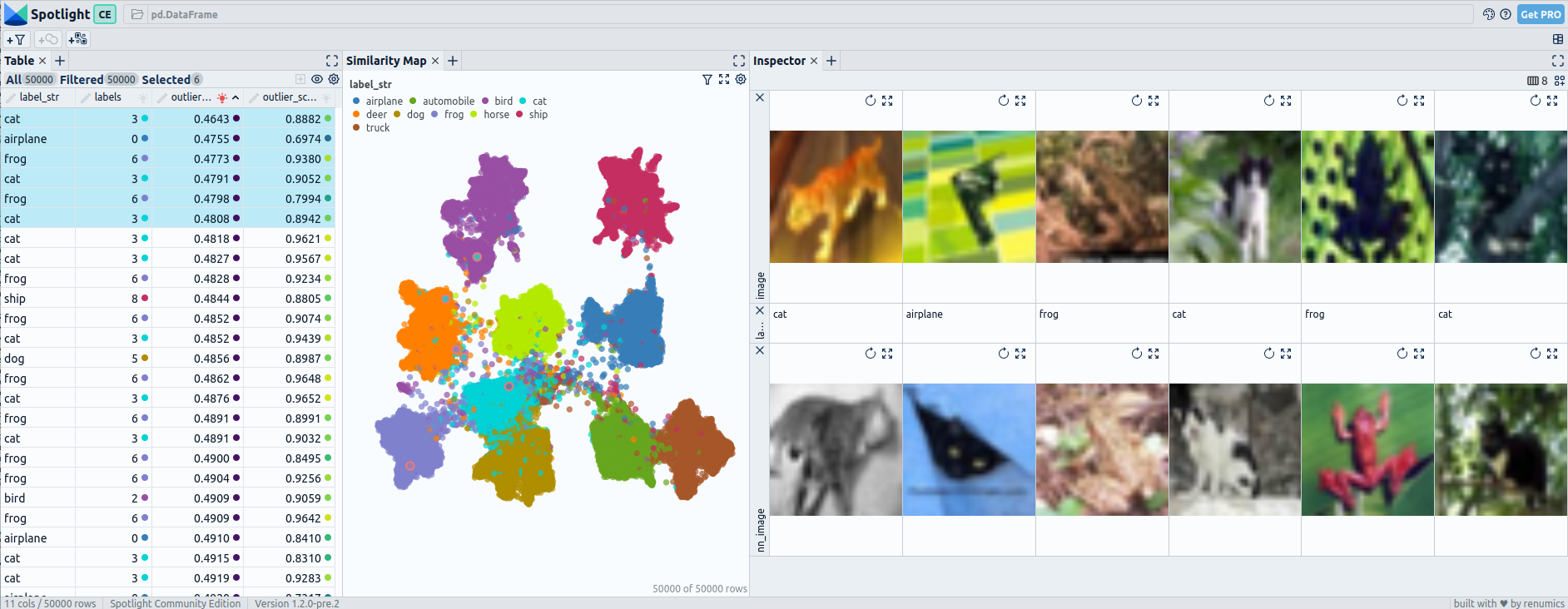
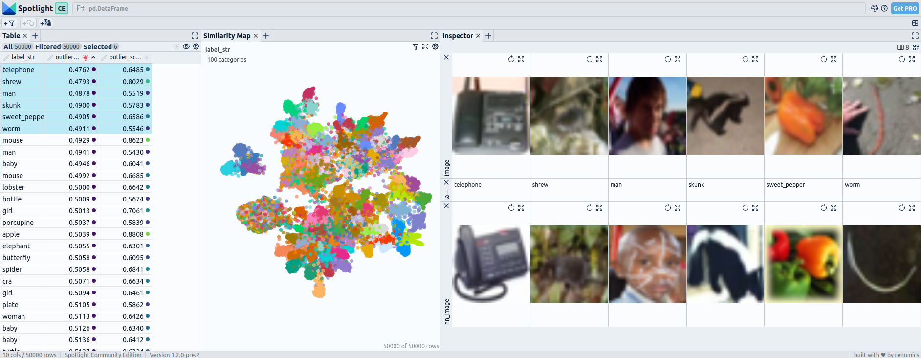
Pre fine-tuning embeddings for CIFAR-10: UMAP and 6 worst outliers — visualized with Spotlight.
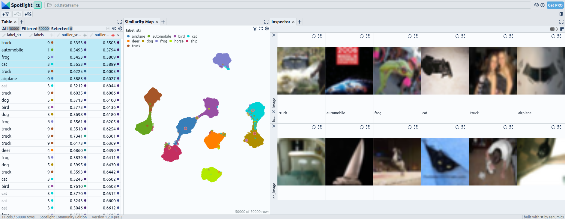
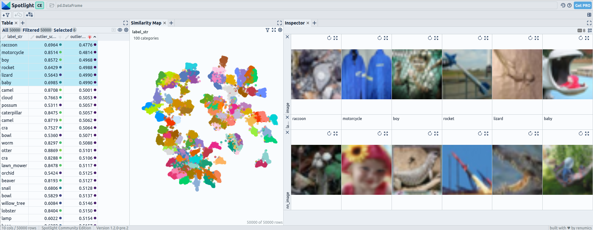
Post fine-tuning embeddings for CIFAR-10: UMAP and 6 worst outliers — visualized with Spotlight.
The UMAP visualization of the embeddings after fine-tuning reveals distinct patterns where certain classes are completely separated from all others, while some may be connected to only one or two other classes.
The outliers detected in CIFAR-10 using pre-fine-tuning embeddings do not appear to be significantly uncommon, as they have relatively similar neighboring images. In contrast, the outliers identified with post-fine-tuning embeddings are distinct and highly uncommon within the dataset.
3.2 CIFAR-100
Load the prepared CIFAR-100 dataset [3] with
from renumics import spotlight
import datasets
ds = datasets.load_dataset("renumics/cifar100-outlier", split="train")
df = ds.rename_columns({"img": "image", "fine_label": "labels"}).to_pandas()
df["label_str"] = df["labels"].apply(lambda x: ds.features["fine_label"].int2str(x))
dtypes = {
    "nn_image": spotlight.Image,
    "image": spotlight.Image,
    "embedding_ft": spotlight.Embedding,
    "embedding_foundation": spotlight.Embedding,
}
spotlight.show(
    df,
    dtype=dtypes,
    layout="https://spotlight.renumics.com/resources/layout_pre_post_ft.json",
    )
or checkout the online demo at huggingface.co/spaces/renumics/cifar100-outlier to examine the outliers:
Pre fine-tuning embeddings for CIFAR-100: UMAP and 6 worst outliers — visualized with Spotlight.
Post fine-tuning embeddings for CIFAR-100: UMAP and 6 worst outliers — visualized with Spotlight.
When examining the embeddings of CIFAR-100, which consists of 100 classes, we observe that even after fine-tuning, there are still more connected classes compared to the pre-fine-tuning embeddings. However, the structure within the embedding space becomes noticeably more defined and organized
The pre-fine-tuning embeddings do not show clear outliers that stand out from their neighboring images, indicating limited effectiveness in outlier detection. However, when utilizing post-fine-tuning embeddings, the performance improves. Out of the six outliers identified, the first three are effectively detected as uncommon within the dataset.
3.3 MNIST
Load the prepared MNIST dataset [4] with
from renumics import spotlight
import datasets
ds = datasets.load_dataset("renumics/mnist-outlier", split="train")
df = ds.rename_columns({"label": "labels"}).to_pandas()
df["label_str"] = df["labels"].apply(lambda x: ds.features["label"].int2str(x))
dtypes = {
    "nn_image": spotlight.Image,
    "image": spotlight.Image,
    "embedding_ft": spotlight.Embedding,
    "embedding_foundation": spotlight.Embedding,
}
spotlight.show(
    df,
    dtype=dtypes,
    layout="https://spotlight.renumics.com/resources/layout_pre_post_ft.json",
)
or checkout the online demo at huggingface.co/spaces/renumics/mnist-outlier to examine the outliers:
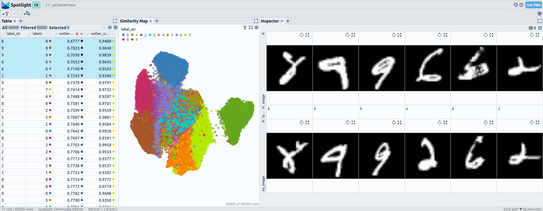
Pre fine-tuning embeddings for mnist: UMAP and 6 worst outliers — visualized with Spotlight.
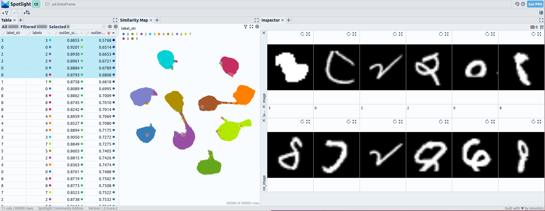
Post fine-tuning embeddings for mnist: UMAP and 6 worst outliers — visualized with Spotlight.
During the fine-tuning of MNIST, the embeddings experience significant changes. Pre-fine-tuning, there may be overlapping regions between different digit classes, making it challenging to distinguish them based on embedding proximity alone. However, after fine-tuning, the embeddings exhibit clearer separations between the digit classes.
The pre-fine-tuning embeddings reveal only one outlier that stands out from the neighboring images, indicating a moderate performance in outlier detection. However, when utilizing post-fine-tuning embeddings, the detection of outliers improves. Approximately 3 to 4 outliers could be identified as highly uncommon within the dataset.
3.4 Beans
Load the prepared beans dataset [3] with
from renumics import spotlight
import datasets
ds = datasets.load_dataset("renumics/beans-outlier", split="train")
df = ds.to_pandas()
df["label_str"] = df["labels"].apply(lambda x: ds.features["labels"].int2str(x))
dtypes = {
    "nn_image": spotlight.Image,
    "image": spotlight.Image,
    "embedding_ft": spotlight.Embedding,
    "embedding_foundation": spotlight.Embedding,
}
spotlight.show(
    df,
    dtype=dtypes,
    layout="https://spotlight.renumics.com/resources/layout_pre_post_ft.json",
)
or checkout the online demo at huggingface.co/spaces/renumics/beans-outlier to examine the outliers:
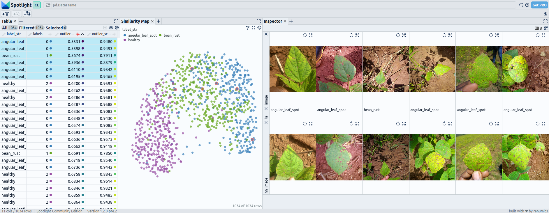
Pre fine-tuning embeddings for beans: UMAP and 6 worst outliers — visualized with Spotlight.
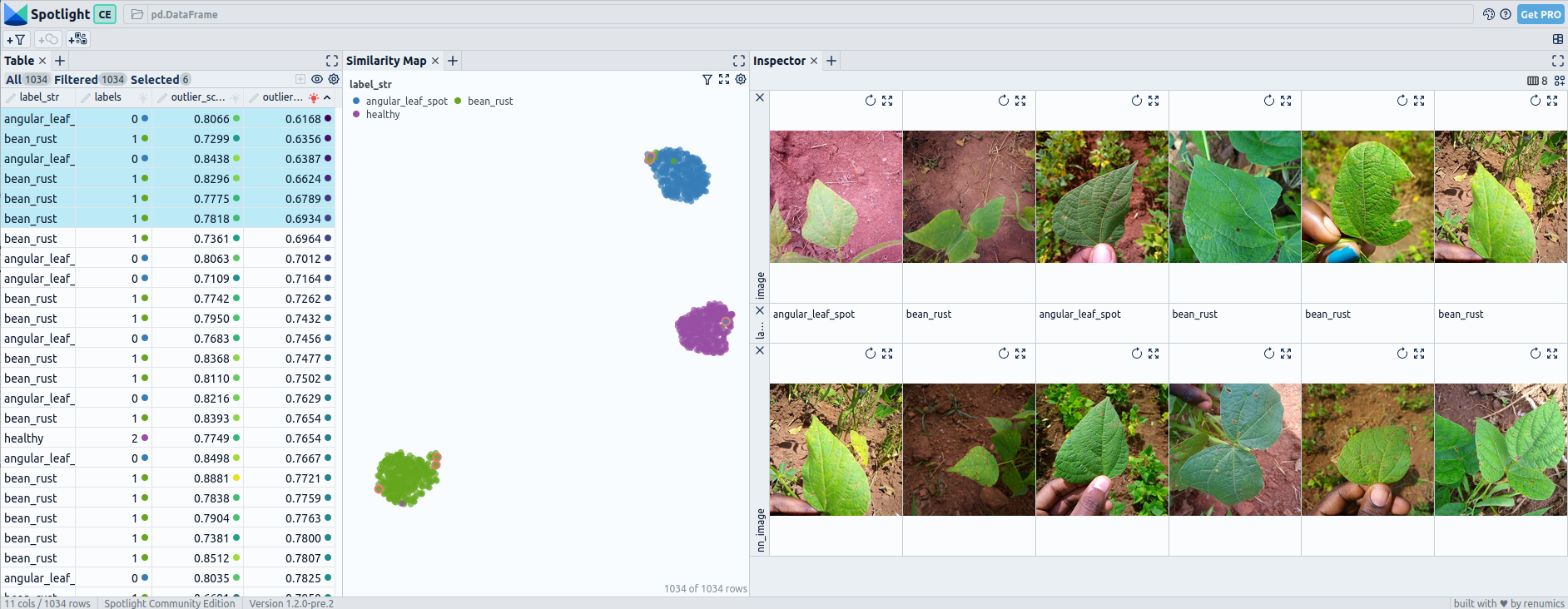
Post fine-tuning embeddings for beans: UMAP and 6 worst outliers — visualized with Spotlight.
In the Beans dataset, after fine-tuning, most of the embeddings exhibit complete separation between the three classes. However, a few cases still show slight overlaps, possibly due to similarities between certain types of beans or misclassifications.
The outlier detection using both pre-fine-tuning and post-fine-tuning embeddings does not yield significant outliers that deviate from the norm. The identified outliers are not distinct or uncommon within the dataset.
4 Conclusion
In conclusion, fine-tuning has a significant impact on embeddings in image classification. Before fine-tuning, embeddings provide general-purpose representations, while after fine-tuning, they capture specific features for the task at hand.
This distinction is clearly reflected in the UMAP visualizations, where post-fine-tuning embeddings exhibit more structured patterns, with certain classes completely separated from others.
For outlier detection, using post-fine-tuning embeddings can be more effective. However, it’s worth noting that calculating outliers based on the probabilities obtained from fine-tuning might yield even better results compared to relying solely on the embeddings.
Both pre-fine-tuning and post-fine-tuning embeddings have their unique strengths and should be used in combination to achieve a comprehensive analysis in image classification and analysis tasks.
References
[1] Alexey Dosovitskiy, Lucas Beyer, Alexander Kolesnikov, Dirk Weissenborn, Xiaohua Zhai, Thomas Unterthiner, Mostafa Dehghani, Matthias Minderer, Georg Heigold, Sylvain Gelly, Jakob Uszkoreit, Neil Houlsby An Image is Worth 16x16 Words: Transformers for Image Recognition at Scale (2020), arXiv
[2] Ze Liu, Yutong Lin, Yue Cao, Han Hu, Yixuan Wei, Zheng Zhang, Stephen Lin, Baining Guo Swin Transformer: Hierarchical Vision Transformer using Shifted Windows (2021), arXiv
[3] Alex Krizhevsky, Learning Multiple Layers of Features from Tiny Images (2009), University Toronto
[4] Yann LeCun, Corinna Cortes, Christopher J.C. Burges, MNIST handwritten digit database (2010), ATT Labs [Online]
[5] Makerere AI Lab, Bean disease dataset (2020), AIR Lab Makerere University