Introduction
As a data scientist or ML engineer, you likely have a vast collection of Jupyter Notebooks and Python scripts to analyze your data. You may even have additional scripts for cleaning data of various types, such as images or audio, and for creating datasets. This can lead to a never-ending search for the ideal tools and the perfect line of code to tackle your current problem.
When you are faced with a problem that has only limited access to labeled data, synthetic data generation comes in handy. Synthetic data overcomes the following problems:
- Time, effort, and costs related to manual or semi-automated gathering and annotation of data
- Bias: e.g., for image data: overrepresented samples
- Availability of data that aligns with your specific problem can be limited due to privacy and competition concerns. Additionally, obtaining samples depicting rare edges is relatively infrequent and can be expensive to generate.
However, synthetic data generation does not come without cost. It requires significant effort in guiding and controlling the generation process. While eliminating biases in datasets is commendable, it is crucial to detect and identify them first. Furthermore, the quality of the generated examples must be validated.
In this article, we will leverage only a single tool for data exploration and curation. We will get a better understanding of an image dataset by interactively exploring structured and unstructured data instead of exhaustively creating visualizations and data reports in the Jupyter Notebook code-block style. Our goal is to derive comprehensible directives for synthetic data generation.
The Challenge
Recently, the first CVPR VISION workshop targeting challenges of vision-based industrial inspection has been hosted. The organizers emphasized a crucial issue:
Modern manufacturing industries are data-rich but label-rare; getting labeled defect data is hard, expensive, and takes a long time, which makes vision-based industrial inspection different from general computer vision tasks.
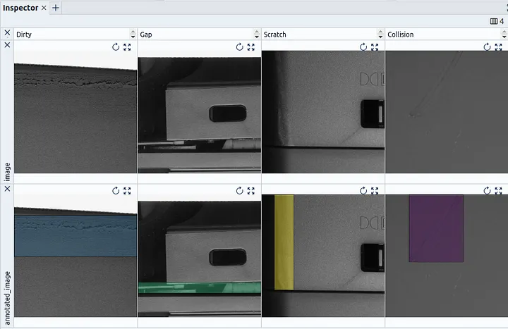 Spotlight’s Inspector Widget lets you examine images and object detection annotations interactively and side-by-side.
To tackle this challenge and enhance defect detection capabilities, a competition has emerged with a primary focus on synthetic data generation. In this competition, participants are provided with a fixed detection algorithm and are tasked with emphasizing the generation of synthetic data to enhance defect detection.
So our setting is clear, we focus on improving a model by tweaking around on the data side — A Data-centric AI approach.
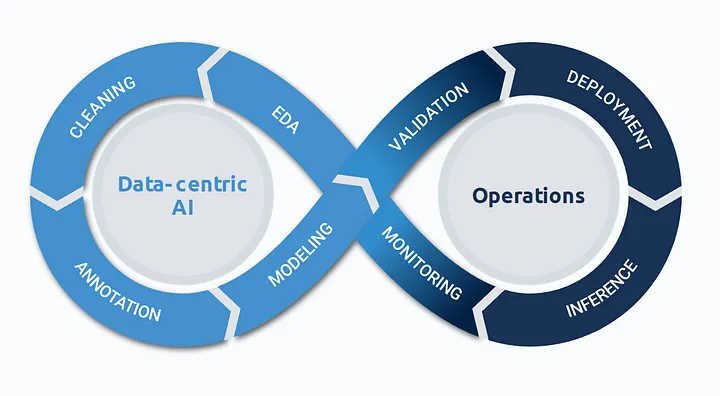 Data-centric AI Flywheel.
If you’re wondering where synthetic data generation fits into the chart: it runs parallel to EDA, Cleaning, and Annotation in an iterative manner. For the generation of additional training data, you should ideally be aware of use-case-specific data distributions, know domain-specific image issues and outliers, and address potential label inconsistencies and edge cases.
Our goal is to understand the underlying domain of data and its (hidden) distribution and get a grasp of the prevalent defect cases. Based on this information, we will make simple directives for data generation, e.g.: Based on observation X, we need to do Y to overcome issue/bias Z.
Our Next Steps:
- Load the image data
- Enrich the data with embeddings and outlier scores for in-depth analysis of unstructured data, in our case images.
- Add pseudo-labels representing the part-category
Preparation
Before we can load the data, we have to install all the necessary Python packages with pip:
pip install renumics-spotlight datasets transformers hnne
The data for VISION Competition Track 2 is accessible for non-commercial use after filling out this form. After downloading and extracting the data, we are loading the images with Hugging Face Datasets into an Image Dataset.
import datasets
# functions from utils package are located at the end of this article
from utils import load_cvpr_track2_dataset, flatten_features, add_bbox_image, create_color_map

path = "/path/to/Console_sliced"
dataset, categories = load_cvpr_track2_dataset(path)
Since Spotlight can load data directly from in-memory Pandas DataFrames and Datasets has a Pandas interface, we are already set up for visual exploration. Yet, we can further enrich the Image Dataset to enable more in-depth investigation.
Note: Although we use a specific dataset for demonstration, all of the techniques presented can be easily applied to your own data. The only prerequisite is that you have references to your image file as an “image” column in a Pandas DataFrame. Optionally, object detection annotation in COCO-Format can be handled in the “objects” column.
Adding Image Embeddings from a Foundation Model
 Spotlight’s Similarity Map projects data points onto a 2D Map: Image Embeddings can be used to analyze the content of images regarding similarity. As we can see, different defect types occur more and less frequently in different regions of the latent space.
Embeddings can help us to analyze unstructured image data. The embeddings from a foundation model offer general-purpose representations of the image content for further analysis in Spotlight.
Learn more about image embeddings in this article from my colleague Markus Stoll.
In the following code section, we enrich our dataset with embeddings, create annotations in image format for visual exploration, and fit the unstructured object detections to our table-like data format.
device = "cuda"
split = "train"

cm = create_color_map([c["name"] for c in categories])
features = dataset["train"].features.copy()
features.update({"annotated_image": datasets.Image()})

# create embeddings with foundation model
split_emb = huggingface_embedding(dataset[split].to_pandas(), modelname="google/vit-base-patch16-224", device=device)

# create annotated images -> save on disk -> save url in DataFrame
annotated_split = dataset[split].map(lambda sample: add_bbox_image(sample, directory=path + "/annotations", color_map=cm), features=features)

# map object detection instances to image samples
df_split = flatten_features(annotated_split.to_pandas())
df_split["split"] = split

# append enriched split data
df = pd.concat([df_split, split_emb], axis=1)
Adding pseudo-labels with Hierarchical Clustering
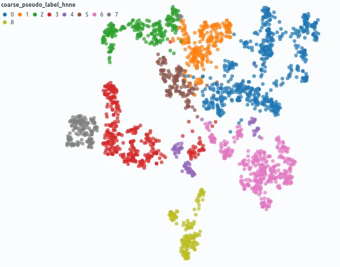 Hierarchical clustering of image embeddings created with a foundation model can be used to group data points based on the image content.
In our case, we do not have any structured information about the content shown in the image (class labels), besides that the picture show sections of the housing of a video game console. Consequently, we integrate pseudo-labels to suggest potential categorization for the part of the console visible in the image.
from hnne import HNNE
import numpy as np

hnne = HNNE()
projection = hnne.fit_transform(np.stack(df["embedding"]), verbose=True)
partitions = hnne.hierarchy_parameters.partitions

df["coarse_pseudo_label_hnne"] = partitions[:, partitions.shape[1] - 1].tolist()
df["fine_pseudo_label_hnne"] = partitions[:, partitions.shape[1] - 2].tolist()
Let’s start Spotlight and explore the training data:
from renumics import spotlight

spotlight.show(df, dtype={"image": spotlight.Image, "annotated_image": spotlight.Image,  "embedding": spotlight.Embedding})
Hint: You can set argument analyze=True in spotlight.show(…). This will automatically detect potential issues in the image dataset with Cleanvision and highlight them in the Spotlight UI.
The Results
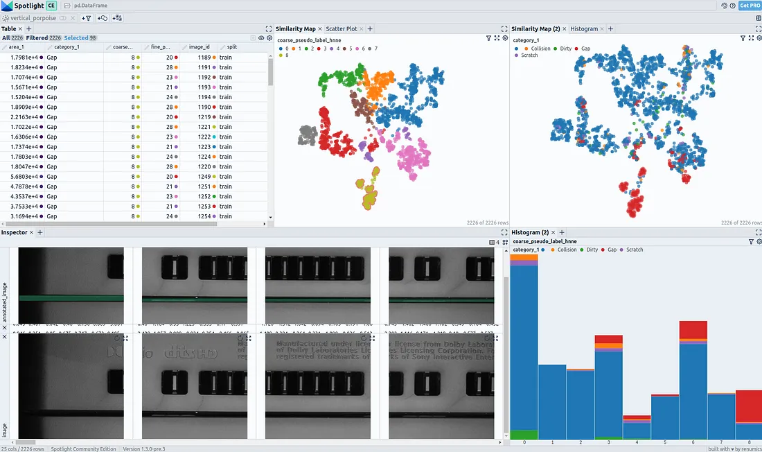
We are now able to explore and analyze our training data interactively with Spotlight’s Widgets. On the Similarity Map, the data points are placed by similarity between image embeddings. As we can see, our applied clustering reflects on regions in the Similarity Map. When we color the data points by defect type, it is observable that there is an unequal distribution for the occurrence of distinctive defect types in embedding space.
This is a hint that there is a hidden stratification of labels regarding image content — in our case parts of the game console housing.
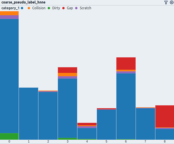 The histogram shows the distribution of data points regarding the coarse pseudo-label colored by the defect type.
Defects do not occur evenly distributed regarding our pseudo-label for the part category, both in terms of frequency and relative distribution.
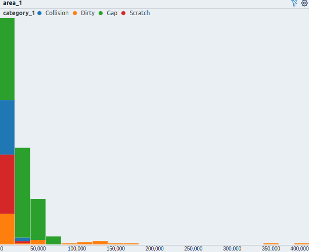 Histogram of defect areas colored by the respective defect type.
The size of a defect (px²) varies for the different defect types. Bigger defects are rather uncommon and only occur for defects of type Dirty.
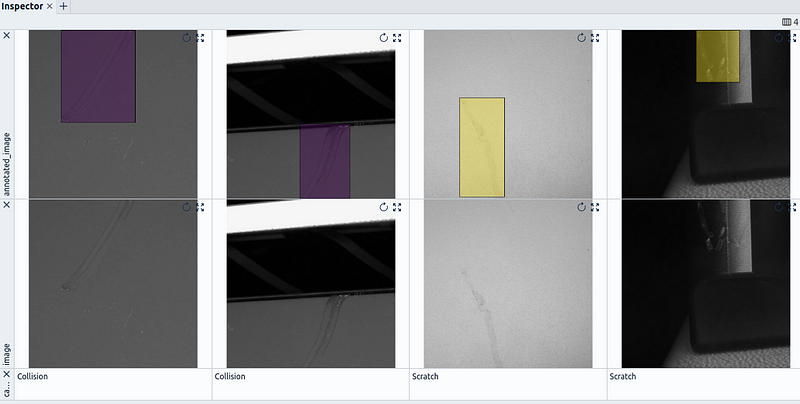 Four data points are displayed in Spotlight's Inspector Widget. Samples with defects of type Scratch and Collision are selected.
Defects of type Scratch and Collision can look very similar. We have to understand the difference between them in order to generate appropriate synthetic samples for each type.
Our key findings:
- Defect distribution is shifted for images of different parts of the case.
- Defects of type Collision, Dirty, and Scratch can appear independently from part geometry — Gap can only occur at shared edges.
- Cluster (1) without any defects exists.
- Data points with pseudo-label 2, 5, 7, and 8 lack defect type Dirty.
- Domain knowledge for the distinction between Collision and Scratch can be helpful.
- Defect types have characteristic sizes.
Critical Segments:
- A: There is a segment of data points including almost exclusively dark images without defects. Many of them appear to be near-duplicates and can probably be removed without losing relevant information.
- B: The segment of images with cooling fins (7) has only four samples with defects (Collision and Scratch).
… There are many more critical segments to find analog to B; go try it yourself.
Based on the findings, we can derive interpretable actions for synthetic data generation. For example:
Based on the observation that there are only a few images with cooling fins and defects (edge case), we need to synthetically create images with cooling fins that have defects of type Scratch, Collision, and Dirty, to overcome the hidden stratification issue.
Conclusion
In this article, we used Spotlight to visually explore an image dataset and understand the hidden distribution regarding image content and label. We enriched the unstructured image data with embeddings and pseudo-labels to uncover critical segments with Spotlight’s Similarity Map and Histogram Widget.