Exploring Underwater Soundscapes with Data-Centric AI

Understanding underwater soundscapes

The oceans are full of sounds. These include well-known signals such as whale calls and ship noise, but also less familiar sounds made by fish and invertebrates, or other still unidentified acoustic events. The analysis of these sounds can provide information which can be used to assess ecosystem health, human impact, and biodiversity.

To study these underwater soundscapes, researchers can use hydrophones that continuously record underwater environments over weeks, months or years. Such deployments can easily generate thousands of hours of audio data per hydrophone that need to be explored, organized, and interpreted.

A public example of this type of large-scale marine acoustic research effort is the Marine SoundLib, developed by the Flanders Marine Institute (VLIZ). The platform provides access to curated underwater sound events and long-term trends of sound levels at different frequency bands across different locations. Researchers can explore marine sound events interactively, including a 2D visualization of all sounds of interest using deep learning embeddings and UMAP [1].

Making sense of these large acoustic datasets remains a major challenge. While machine learning methods for bioacoustics have advanced significantly in recent years, many practical workflows still require extensive manual exploration and expert interpretation. In many cases:

• Researchers do not have enough labelled annotations of a target sound to train machine learning models.
• Researchers first need to determine whether different sound types can even be distinguished reliably.
• Most sound events in the soundscape are of unknown origin.

As a result, marine bioacoustics increasingly depends on iterative workflows that combine machine learning with human-guided exploration and curation.

In this blog post, we, Renumics together with the Flanders Marine Institute (VLIZ), outline how data-centric workflows and interactive curation tools such as Renumics Spotlight can help researchers explore underwater soundscapes more efficiently, organize large acoustic datasets, and iteratively improve detector development and scientific analysis.

But what does such an iterative workflow actually look like in practice?

An iterative workflow for exploring and organizing sounds

Curating bioacoustics data is no waterfall. The challenges outlined above — too few labels, uncertain class boundaries, unknown sound origins — all share a root cause: you cannot annotate what you do not yet understand. The practical response is an iterative workflow where each step reshapes the next. A typical cycle passes through five stages:

• Enrich: Bring the data into an explorable format by computing features such as statistical summaries and embeddings from pre-trained acoustic models. Without explorable features, thousands of hours of audio remain opaque.
• Explore: Investigate the enriched data to discover structure: which sound types are present, how they cluster, where the boundaries lie.
• Annotate: Label the data, informed by what exploration revealed. Select training examples and define splits for an acoustic event detector.
• Train: Fit a model. At this stage the model is not the final detector. It is a diagnostic tool that reveals where the real challenges are.
• Evaluate: Inspect the model’s errors and confidence scores. These become signals for the next round of exploration, e.g. by showing ambiguous sounds, wrongly annotated sounds etc.

The value of this workflow is in the iteration, not in any single step. Each pass through the loop refines the researcher’s understanding of the data, which in turn makes the next pass more targeted.

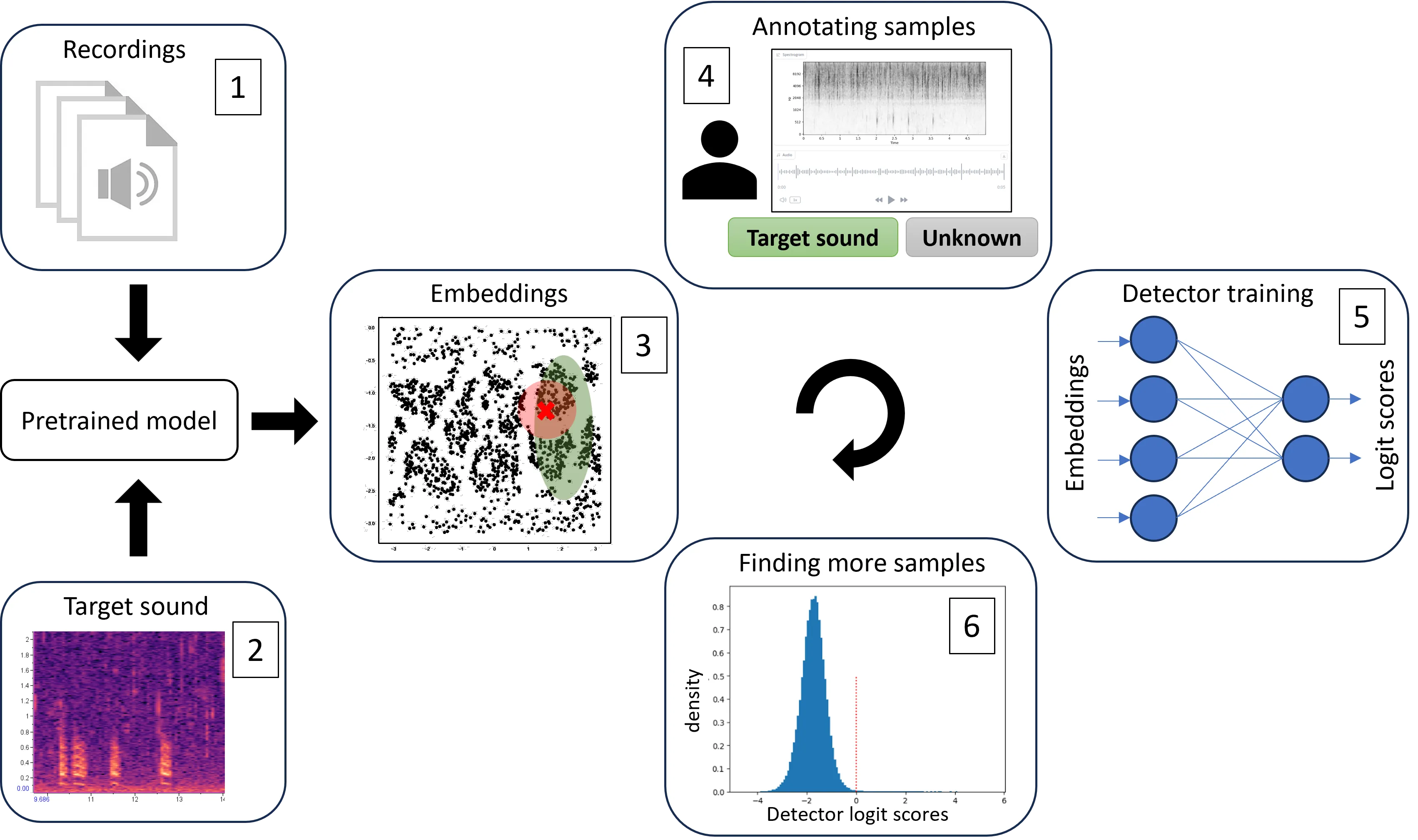Figure 1: An active-learning cycle for bioacoustic data curation, after Bordoux et al.: recordings (1) and a target sound reference (2) are enriched with embeddings from a pre-trained model (3), annotated by a human expert (4), used to train a detector (5), and the detector’s confidence scores guide the selection of new samples for the next round (6). In practice, an exploration phase between computing embeddings and annotating, investigating what the clusters reveal before committing to labels, is often the most consequential part of the cycle.

A practical example of this application would be to decide on an active learning sampling strategy, such as the one proposed in Bordoux et al. (2026) [9]. Several technical building blocks support this loop. Embedding models pre-trained on acoustic data (such as Perch [2], SurfPerch [3] or BirdNet [4]) project raw audio into a space where similar sounds sit near each other. Dimensionality reduction with UMAP makes that space visually navigable, and model-driven diagnostics (confidence scores, error analysis) turn a trained model’s weaknesses into a guide for the next iteration. This process helps researchers understand which samples lead to improved model performance.

The question, then, is what one turn of this loop looks like in practice?

How Renumics Spotlight supports human-in-the-loop bioacoustics — a concrete example

Why this example

We use a public benchmark so that readers can follow along with the same data: the BioDCASE 2026 Task 2 challenge, detecting calls of Antarctic blue and fin whales. It mirrors the real difficulties of Passive Acoustic Monitoring. The target calls are present only about 6% of the time, spread across many sites and years with highly variable soundscapes. The data is the IWC-SORP AcousticTrends_BlueFinLibrary recordings sampled at just 250 Hz, with seven strongly-labelled call types (blue-whale A/B/Z and D, and three fin-whale types). The same approach applies to the real research cases that follow below.

We deliberately stop short of building a detector. The goal is to show the part Spotlight is built for: getting a feel for unfamiliar data and seeing where a model will struggle. These are the early, decisive loops of the curation process described above.

Step 1: Turn annotations into an explorable dataset

Each annotated call becomes one row. We cut the clip from its recording and save an audible version (these calls are infrasonic, so we replay them 16x faster so they can be heard). We also compute a compact “fingerprint” of the call’s frequency shape, but we do not store a spectrogram image: Spotlight draws one from the audio on the fly.

sound, rate = librosa.load(recording, sr=None, offset=start, duration=length)
sf.write(audio_file, sound, rate * 16)  # 16x faster -> infrasound becomes audible
# Compute a spectrogram only to build a compact fingerprint: loudness per frequency in the
# first half vs. the second half of the call, so calls that sweep up or down look different
# from flat tonal calls. (small window because the calls are very low-frequency, at 250 Hz)
spectrogram = librosa.power_to_db(
    librosa.feature.melspectrogram(y=sound, sr=rate, n_fft=256, hop_length=32, n_mels=32)
)
half = spectrogram.shape[1] // 2
fingerprint = np.concatenate([spectrogram[:, :half].mean(axis=1), spectrogram[:, half:].mean(axis=1)])

Collected into one dataframe alongside a few numbers taken straight from the annotations (duration_s, freq_low_hz, freq_high_hz, site), opening it is a single call:

spotlight.show(
    data,
    dtype={"audio": spotlight.Audio, "frequency_profile": spotlight.Embedding},
)

Spotlight links every data type in one view. For any audio column it renders both a player with a waveform and a spectrogram, on the fly. You get the visual without ever storing an image, alongside the high-dimensional embedding and ordinary scalar metadata, all linked across every chart.

Step 2: Explore the calls and build intuition

Color the Similarity Map (a UMAP projection of the fingerprint) by call_type. Structure appears immediately: the low-frequency tonal blue-whale calls (A/B/Z, all around 16—28 Hz) gather in one region, while the short, higher-frequency downsweeps (blue-whale D and the fin-whale 40 Hz downsweep, ~50—84 Hz) sit apart. Brush a group, open the Inspector, and you can view each call as a player, as a spectrogram, and listen to it.

It is just as instructive to see what the simple fingerprint cannot separate. The blue-whale call types differ by how much of the same descending unit they contain. The A-call covers only the top part (~24—27 Hz); the B- and Z-calls extend the sweep down toward 16 Hz. As a result, all three overlap heavily on the map. That observation sets up the next step.

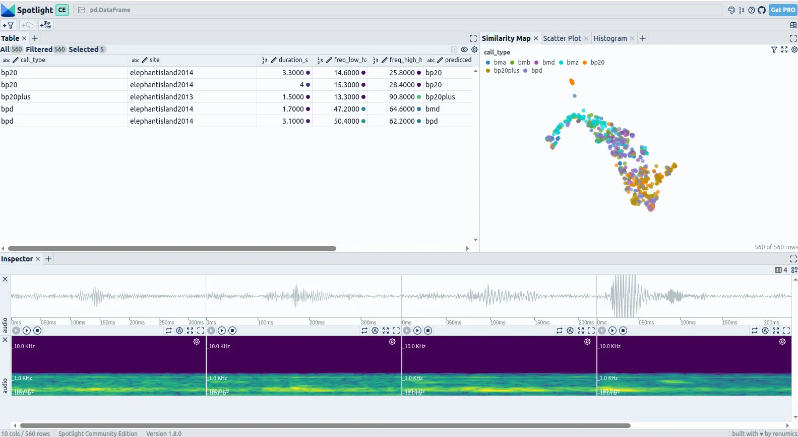Figure 2: Similarity Map coloured by call type, with the Inspector showing one call as a player and as a Spotlight-rendered spectrogram. Blue-whale tonal calls cluster at low frequency; the short downsweeps separate out. A/B/Z overlap because they share the same descending sweep.

Takeaway: before any training, Spotlight already shows which call types are easy to distinguish and which share too much acoustic structure to be separated by simple features.

Step 3: Find the detector’s blind spots

Now train a small model on just three human-readable numbers and write its guess, confidence, and correctness back into the same table:

features = data[["duration_s", "freq_low_hz", "freq_high_hz"]]
model = RandomForestClassifier(n_estimators=200, random_state=0)
probabilities = cross_val_predict(model, features, data.call_type, cv=5, method="predict_proba")
class_order = sorted(data.call_type.unique())
data["predicted"] = [class_order[i] for i in probabilities.argmax(axis=1)]
data["confidence"] = probabilities.max(axis=1).round(2)
data["correct"] = data.predicted == data.call_type

Now re-open Spotlight with the enriched table:

spotlight.show(
    data,
    dtype={"audio": spotlight.Audio, "frequency_profile": spotlight.Embedding},
)

Those three numbers alone reach 81% accuracy across seven classes. The valuable question is where it fails, and in Spotlight that is a few clicks on the same enriched table:

• Color by correct and open the Confusion Matrix. Errors concentrate on the acoustically overlapping pairs: the fin-whale 40 Hz downsweep and the blue-whale D-call (both ~50—84 Hz, ~1—2 s) swap in both directions, and the blue-whale B- and Z-calls trade places. The well-separated classes stay near-perfect (blue-whale A 98%, fin 20 Hz pulse 99—100%), while the overlapping downsweeps fall to 56—69%.
• Color by confidence (or filter confidence < 0.7). The model’s own uncertainty is a reliable guide: wrong predictions have a median confidence of 0.66 versus 0.90 for correct ones. The lowest-confidence calls form a short, high-value listening queue.
• Group by site. The error rate ranges from 0% at one deployment to 31% at Casey 2014 and 25% at Maud Rise 2014. This is not noise: the challenge organisers note that at exactly these sites a strong chorus band of overlapping fin-whale pulses and blue-whale Z-calls makes single calls hard to isolate. Spotlight surfaces that documented difficulty straight from the data. You can jump to those calls and hear the chorus yourself.

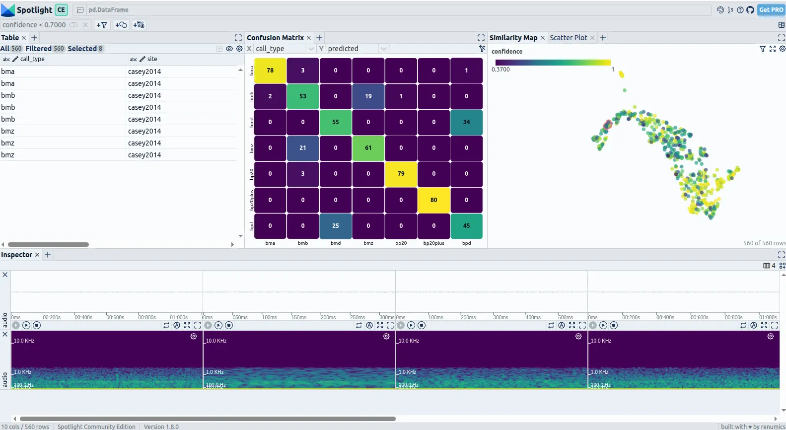Figure 3: Similarity Map coloured by confidence with confidence < 0.7 active, Inspector on a low-confidence downsweep. Low-confidence calls cluster exactly where the downsweep classes overlap: the model’s uncertainty points straight at the genuinely ambiguous calls.

Takeaway: the same dataframe, now carrying model outputs, becomes an error-analysis tool. Every conclusion came from colouring, filtering, and listening. No extra code.

What this demonstrates

This is the enrich-explore-annotate-train-evaluate loop in miniature: enrich, explore, model, inspect failures, all in one interactive view. We learned which call types are inherently confusable and which recording sites deserve closer annotation review before committing to a heavy detector. These are the kinds of early insights that keep a curation project moving.

The same patterns show up in real ongoing research. In the following case studies, researchers across marine science applied this approach to their own data, and in each case the decisive insights came from exploring and understanding the data, often before any model was trained.

Try it yourself. The full script is below. With the dataset in data/train, run python blog_spotlight_demo.py; Spotlight opens in your browser. In the Inspector, add an AudioView and a SpectrogramView on the audio column. With no domain features at all, you can even let Spotlight embed the audio for you: spotlight.show(data, embed=["audio"]).

"""Explore Antarctic whale calls with Renumics Spotlight (BioDCASE Task 2)."""
from pathlib import Path
import librosa
import numpy as np
import pandas as pd
import soundfile as sf
from renumics import spotlight
from sklearn.ensemble import RandomForestClassifier
from sklearn.model_selection import cross_val_predict

DATA = Path(__file__).parent / "data" / "train"
CLIPS = Path("/tmp/whale_clips")
CLIPS.mkdir(exist_ok=True)

# 1. Load every annotated call into one table, keep 80 examples per call type.
annotations = pd.concat(
    pd.read_csv(p, parse_dates=["start_datetime", "end_datetime"])
    for p in (DATA / "annotations").glob("*.csv")
)
calls = annotations.groupby("annotation", group_keys=False).sample(
    80, random_state=0
).reset_index(drop=True)


def file_start(filename):
    """Recordings are named after their start time, e.g. 2015-02-04T03-00-00_000.wav."""
    day, clock = filename.replace(".wav", "").rsplit("_", 1)[0].split("T")
    return pd.Timestamp(f"{day}T{clock.replace('-', ':')}")


# 2. Cut each call out of its recording, save an audible clip, and build a frequency fingerprint.
audio_files, frequency_profiles = [], []
for i, call in calls.iterrows():
    recording = DATA / "audio" / call.dataset / call.filename
    start = max(0, (call.start_datetime - file_start(call.filename)).total_seconds() - 1)
    length = (call.end_datetime - call.start_datetime).total_seconds() + 2
    sound, rate = librosa.load(recording, sr=None, offset=start, duration=length)

    # These calls are infrasound (~20 Hz), so play them back 16x faster to make them audible.
    # Spotlight shows the player AND a spectrogram straight from this audio - no image needed.
    audio_file = CLIPS / f"{i}.wav"
    sf.write(audio_file, sound, rate * 16)

    # We still compute a spectrogram in memory, only to build a compact frequency fingerprint:
    # how loud each frequency is in the first half vs the second half of the call, so calls
    # that sweep up or down look different from flat tonal calls.
    # (small window because the calls are very low-frequency, recorded at just 250 Hz)
    spectrogram = librosa.power_to_db(
        librosa.feature.melspectrogram(y=sound, sr=rate, n_fft=256, hop_length=32, n_mels=32)
    )
    half = spectrogram.shape[1] // 2
    fingerprint = np.concatenate(
        [spectrogram[:, :half].mean(axis=1), spectrogram[:, half:].mean(axis=1)]
    )

    audio_files.append(str(audio_file))
    frequency_profiles.append(fingerprint)

data = pd.DataFrame({
    "call_type": calls.annotation,
    "site": calls.dataset,
    "duration_s": (calls.end_datetime - calls.start_datetime).dt.total_seconds().round(1),
    "freq_low_hz": calls.low_frequency,
    "freq_high_hz": calls.high_frequency,
    "audio": audio_files,
    "frequency_profile": frequency_profiles,
})

# 3. Train a simple model on the easy-to-read numbers and write its guess back into the same table.
features = data[["duration_s", "freq_low_hz", "freq_high_hz"]]
model = RandomForestClassifier(n_estimators=200, random_state=0)
probabilities = cross_val_predict(model, features, data.call_type, cv=5, method="predict_proba")
class_order = sorted(data.call_type.unique())
data["predicted"] = [class_order[i] for i in probabilities.argmax(axis=1)]
data["confidence"] = probabilities.max(axis=1).round(2)
data["correct"] = data.predicted == data.call_type

# 4. Open everything in Spotlight: audio (player + built-in spectrogram), the frequency-profile
#    map, and the model's mistakes.
spotlight.show(
    data,
    dtype={
        "audio": spotlight.Audio,
        "frequency_profile": spotlight.Embedding,
    },
)

Case studies from marine research

The benchmark walkthrough demonstrated the data-centric loop on a known dataset. The three case studies below show the same approach applied to real, ongoing research: unknown sound discovery in the North Sea, species-level call separation for blue and fin whales, and plankton image classification. The first two are acoustic; the third extends the workflow to visual data, showing that because embeddings represent any data type in a shared geometric space, the approach is modality-agnostic.

Unknown North Sea sound clustering

For some marine ecosystems, very little is known about their biological sounds. Since 2020, the bioacoustics team at the Flanders Marine Institute (VLIZ) has been collecting underwater sound from the Belgian Part of the North Sea. Each recording typically spans several months, making it impossible to listen through everything manually. In many cases, the team did not even know which sounds were of interest.

Therefore, before proceeding to develop sound-specific ML models, we decided to explore the present sounds by first detecting any “salient” events, and afterwards clustering them using embeddings extracted from a pre-trained model (BioLingual [5]). Then the spatio-temporal patterns of the found clusters can be analyzed (see Figure 4). For the exploratory analysis of this study, we used Spotlight to interactively visualize the obtained clusters in the embedding space.

This allowed us to find a clear split between two sounds until then confused, the “squeaking chain” and the “jingle bell”, which before seemed to be harmonics of one same class but turned out to be two distinct clusters because of their very clear frequency range [6].

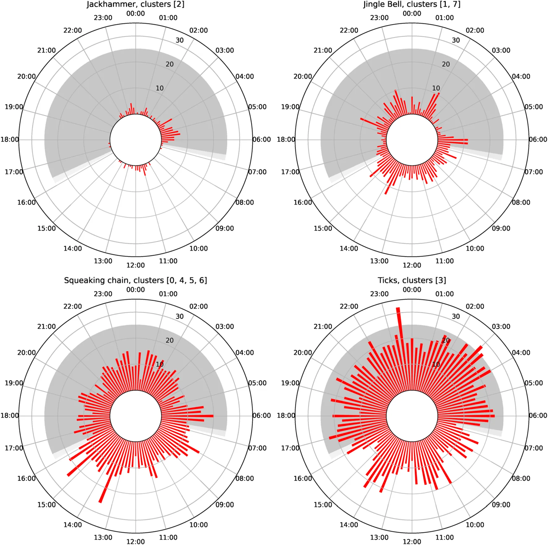Figure 4: Daily activity patterns of four sound clusters found in the Belgian Part of the North Sea. Each cluster shows a distinct temporal signature.

These results led directly to the development of the Marine Sound Library, a collaborative curated library that aims to become the European hub for underwater sounds. The SoundLib, introduced at the beginning of this post, grew directly out of this exploratory work. In the future, we expect that the tool allows researchers the option of checking if a novel sound was already detected somewhere else by another researcher by assessing whether it falls close to other already identified sounds in the embedding space.

To populate the SoundLib, the VLIZ team analysed all events found in the data so far, both manually and automatically detected, producing new and revised classifications of the data (Figure 5) [7].

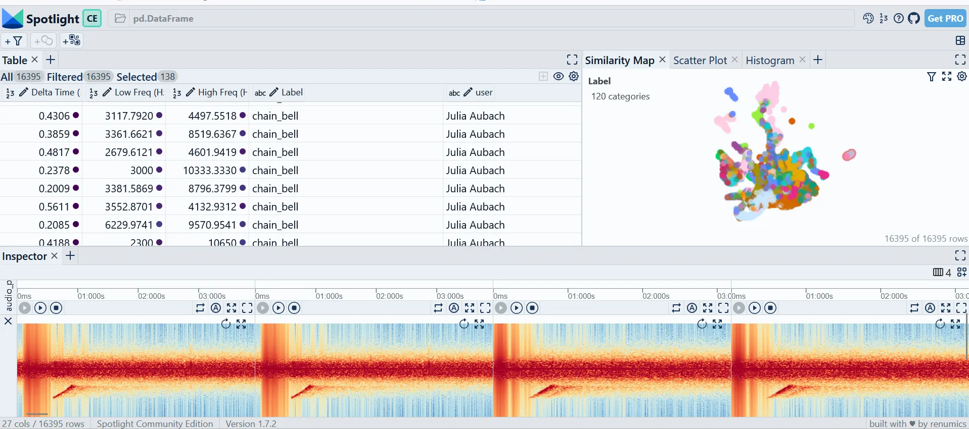Figure 5: All annotated events from the Belgian Part of the North Sea explored in Spotlight.

Whale-call separation

Can blue-whale and fin-whale FM downsweeps be separated by their acoustic features alone? The two call types are so similar that to this day, scientists are not sure how to reliably distinguish them. For long-term monitoring, this matters: the two species need to be tracked separately.

Svenja Wöhle and colleagues at AWI set out during her PhD to find a reliable way of telling these calls apart [8]. The challenge is that even though recordings with both species exist, we rarely know for sure which of the two is vocalising at any given moment.

The team started with a small subset of D-tag recordings (acoustic loggers attached directly to the whale’s skin with a suction cup). Since the recorder is on a known animal, the caller’s species is certain. This subset served as a starting point to explore whether the two species produce acoustically separable signals.

In the projection of the D-tag data (Figure 6), two distinct clusters appear when deep-learning features are used. With Raven features and the same unsupervised approach, however, there is an area of overlap. The deep-learning features provide cleaner separation.

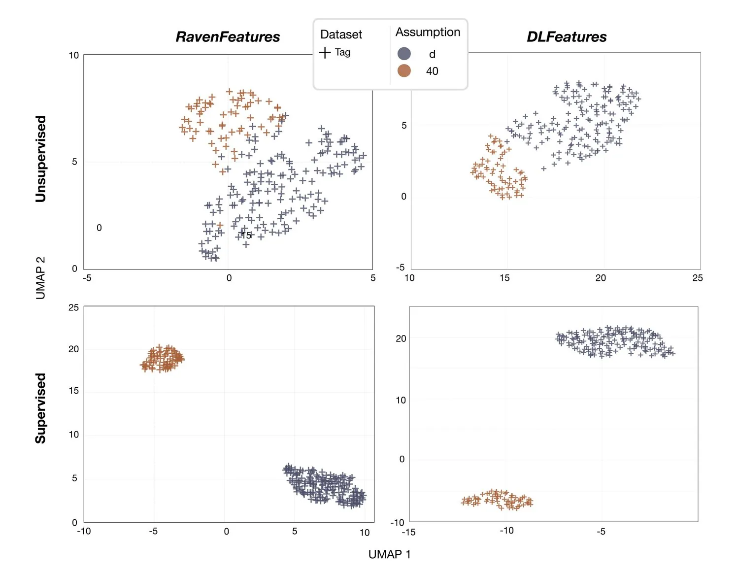Figure 6: Projection of D-tag data for the two species. Left: deep-learning features produce two non-overlapping clusters. Right: Raven features show partial overlap.

The team then projected long-term manually annotated FM events (labelled “FM” because the corresponding species is unknown) together with the D-tag data onto the same embedding space (Figure 7). The Raven features separate most calls, but some events still fall between the two clusters. The deep-learning features are the more reliable option for obtaining a clear separation across all calls.

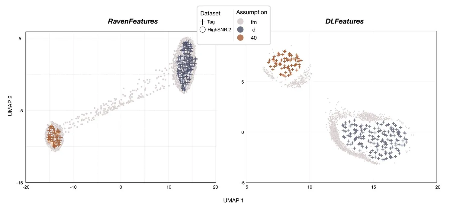Figure 7: UMAP projection of long-term FM detections together with the D-tag data. Deep-learning features maintain cleaner cluster separation than Raven features even with the larger, noisier dataset.

The finding is honest: deep-learning embeddings separate these calls better than traditional acoustic descriptors, but not perfectly. Some events remain genuinely ambiguous even with the best available features.

Plankton imaging

The embedding-driven workflow is not limited to acoustic data. Because embeddings represent any data type in a shared geometric space, the same approach works for images.

In plankton image classification, some particle types look almost identical to human annotators, making consistent labelling based on image appearance alone difficult [11]. To improve the quality of training labels, the team combined image data with particle-level metrics, and used Spotlight to project all samples into a UMAP embedding space and look for hidden structure within existing classes.

This approach helps reveal meaningful subgroups that may otherwise remain unnoticed during manual annotation. Such subclasses are typically more homogeneous and can therefore be learned more effectively by convolutional neural networks (CNNs), leading to improved classification performance.

As an example, what had been labelled as a single class turned out to contain two. The original cnidaria class separated into two distinct clusters, subsequently defined as cnidaria 1 and cnidaria 2 (Figure 8B). The split was not visible during manual annotation but became clear in the embedding space.

The projection also revealed labelling inconsistencies: several samples originally labelled cnidaria 1 fell squarely within the cnidaria 2 cluster. This kind of quality control, catching misassigned labels by their position in feature space, would be difficult to achieve through manual review alone.

Furthermore, Spotlight allows users to inspect individual particle descriptors, such as eccentricity, and visualize their distribution across samples (Figure 8A). This facilitates the identification of subtle morphological differences between particles and provides additional guidance for refining class boundaries and creating biologically meaningful subclasses.

The payoff: By generating more consistent and homogeneous training categories, this process contributes to improved CNN performance and a better separation of classes in the learned feature space.

The classification problem had been partly a labelling problem all along.

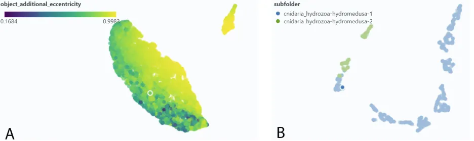Figure 8: UMAP-based intra-class clustering, with each dot representing one image in a similarity map. A: eccentricity values within a single taxon reveal internal structure that supports finer class boundaries. B: the cnidaria class splits into two distinct clusters (green: cnidaria 1, blue: cnidaria 2).

Towards scalable and reusable marine AI workflows

Marine bioacoustics lags behind its terrestrial counterpart. While bird-song classifiers can draw on large, well-annotated public datasets, underwater acoustics has no equivalent. Annotated marine recordings remain scarce, fragmented across institutions, and often limited to a handful of well-studied species.

The three case studies in this post illustrate what becomes possible when data exploration and machine learning work together. In the North Sea, pre-trained embeddings and interactive clustering revealed consistent sound types in the data. For whale calls, deep-learning features provided the separation that traditional acoustic descriptors could not. For plankton, exploring the embedding space uncovered hidden subclasses and labelling errors that, once corrected, improved CNN performance. In each case, novel ML representations made the data explorable, and interactive tools made that exploration actionable.

This combination of domain expertise, modern representations like embeddings, and data-centric exploration tooling is a promising and still underexplored direction for the field. Marine bioacoustics is increasingly becoming a data exploration and curation challenge alongside the model training challenge, and the two reinforce each other: better understanding of the data leads to better models, and model outputs (confidence scores, error patterns) guide the next round of exploration.

Future workflows will be deeply iterative, cycling through the enrich-explore-annotate-train-evaluate loop described earlier with increasing precision on each pass. Representation learning, embedding-space exploration, and metadata-aware analysis are becoming central tools for navigating large collections of underwater recordings. Interactive curation lets researchers see what is in their data before committing to labels or training pipelines.

At the same time, current tooling still has real limitations. Scaling to months of continuous audio per hydrophone remains difficult. Handling streaming acoustic data in near-real-time is not well supported. No single tool seamlessly switches between the continuous-recording view and the extracted-event view. In practice, researchers piece together Raven Pro (or other similar software such as APLOSE [12] or Triton [13]) for annotation, Spotlight for embedding-based exploration and model diagnostics, several python or R packages for analysis (see list of bioacoustics software) and custom scripts to connect them. That fragmentation slows down work that is already data-limited.

Initiatives like the Marine Sound Library point in a promising direction: collaborative, curated platforms where a researcher encountering an unfamiliar sound can check whether it has already been identified elsewhere. Tighter integration between specialised bioacoustics tools and interactive, data-centric AI workflows would make the iterative cycle faster and more accessible to researchers who are not machine-learning specialists. The marine research community and the data-centric AI community have much to build together. The oceans have more to tell us.

References

1. McInnes, L., et al. “UMAP: Uniform Manifold Approximation and Projection for Dimension Reduction.” arXiv:1802.03426, 2020.
2. Merriënboer, B. van, et al. “Perch 2.0: The Bittern Lesson for Bioacoustics.” arXiv:2508.04665, 2025.
3. Williams, B., et al. “Using Tropical Reef, Bird and Unrelated Sounds for Superior Transfer Learning in Marine Bioacoustics.” Philosophical Transactions of the Royal Society B, vol. 380, no. 1928, 2025. doi:10.1098/rstb.2024.0280.
4. Kahl, S., et al. “BirdNET: A Deep Learning Solution for Avian Diversity Monitoring.” Ecological Informatics, vol. 61, 2021. doi:10.1016/j.ecoinf.2021.101236.
5. Robinson, D., et al. “Transferable Models for Bioacoustics with Human Language Supervision.” arXiv:2308.04978, 2023.
6. Parcerisas, C., et al. “Machine learning for efficient segregation and labeling of potential biological sounds in long-term underwater recordings.” Frontiers in Remote Sensing, vol. 5, 2024. doi:10.3389/frsen.2024.1390687.
7. Calonge, A., Parcerisas, C., Schall, E. and Debusschere, E. “Revised clusters of annotated unknown sounds in the Belgian part of the North Sea.” Frontiers in Remote Sensing, vol. 5, 2024. doi:10.3389/frsen.2024.1384562.
8. Wöhle, S., Parcerisas, C., Buchan, S., Calambokidis, J., Stafford, K. M. and Schall, E. “Searching for separation between frequency-modulated calls of blue and fin whales.” Submitted to Scientific Reports (under review).
9. Bordoux, V., Parcerisas, C., Debusschere, E., Jalmby, M., Murk, A. J. and van der Ven, R. M. “Rapid Fish Sound Detection Using Human-in-The-Loop Active Learning.” Ecological Informatics, 2026. doi:10.1016/j.ecoinf.2026.103874.
10. Decrop, W., Deneudt, K., Parcerisas, C., Schall, E. and Debusschere, E. “Transfer Learning for Distance Classification of Marine Vessels Using Underwater Sound.” IEEE Journal of Selected Topics in Applied Earth Observations and Remote Sensing, vol. 18, pp. 19710—19726, 2025. doi:10.1109/JSTARS.2025.3593779.
11. Mortelmans, J., Decrop, W., Deneudt, K. “Semi-automated pipeline for Plankton Imager (Pi-10) imaging: classification, morphometry and data standards.” In preparation.
12. Keribin, E., Morin, E. and Vovard, R. “APLOSE: a scalable web-based annotation tool for marine bioacoustics.” doi:10.5281/zenodo.10467999.
13. Marine BioAcoustics Research Collaborative. “Triton Software Package (Version 1.0.2).” GitHub.